

Option pricing has long been a significant topic of research in quantitative finance, each underlying has its own intricacies which require a nuanced approach.
Before delving into the rabbit hole, let’s simply look at what an option premium consists of:
Option premium = Intrinsic value + extrinsic value
Intrinsic value is the difference between the underlying spot price and the strike price. Any option that’s out of the money (OTM) has 0 intrinsic value. Formulas:
- Call= current stock price − strike price
- Put= strike price − current stock price
Extrinsic value is any extra value it has when intrinsic value is taken out of the option price.
- Extrinsic value = Option Premium – Intrinsic Value
The extrinsic value of an option premium is where things get more interesting as it consists of a variety of different components:
- Time value is the days left to expiry, with the belief that the longer the length of time until the expiry of the contract, the greater the time value.
- Price of the underlying
- Strike
- Volatility
- Dividends
For anyone who has used the Black-Scholes model in the past, you may notice a lot of common parameters.
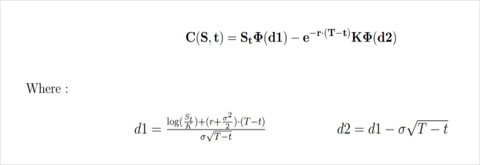
C = call option price
N = CDF of the normal distribution
S_t = spot price of an asset
K = strike price
r = risk-free interest rate
t = time to expiry
σ = volatility of the asset
In most cases anyone who’s looking to price a vanilla option will likely use the black-scholes model. Although the model holds up remarkably to this day, the dynamic nature of financial markets appears to have caused some underlying flaws in the assumptions, which we’ll delve into below. While these assumptions are known and have been covered extensively in plenty of research papers, we had the opportunity to encounter them firsthand while building the Laevitas options calculator.
Implied Volatility
The main driver behind an options price is volatility, whether you’re taking a directional view on an underlying or not, if you’re buying/selling an option you’re largely betting on volatility. Implied volatility is a forecast of how much the price of an asset will move over a given period of time. For European options, the period is the life of the contract. Theoretically, it’s the measure of the market’s expectations for how risky an option is. The Black-Scholes implied volatility σBS(K,T) of the option is defined as the value of the volatility parameter that equals the market price with the price given by the Black-Scholes formula.
Since the crash of 1987, options market participants made the observation that implied volatilities are not constant in contradiction with the Black-Scholes model. It is a necessity to model the implied volatility in order to understand the dynamics of the options market.
∃!σBSt (K,T) > 0
CBS(St,K,T,σBS) = Ct(K,T)
For a fixed strike (K) and expiry (T), one is dealing with a stochastic process. For a fixed t, the value depends fully on the characteristics of the option. The multivariate function:
σBSt : (K,T)→σBSt (K,T)
is known as the Implied Volatility Surface (IVS) at a date t. With the BSM assumptions we would have a constant Implied Volatility surface for every strike and expiry date as displayed below:
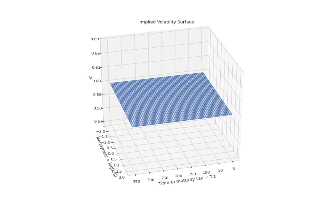
Fig 1 : Implied Volatility Surface in a Black-Scholes world
The implied volatility surface as seen in the market presents some characteristics that are far from the non realistic assumptions of the BSM model as we discussed before. This can cause overpricing or underpricing of options depending on market conditions. However when fitting the Implied Volatility surface using market data, one can obtain the following surface:
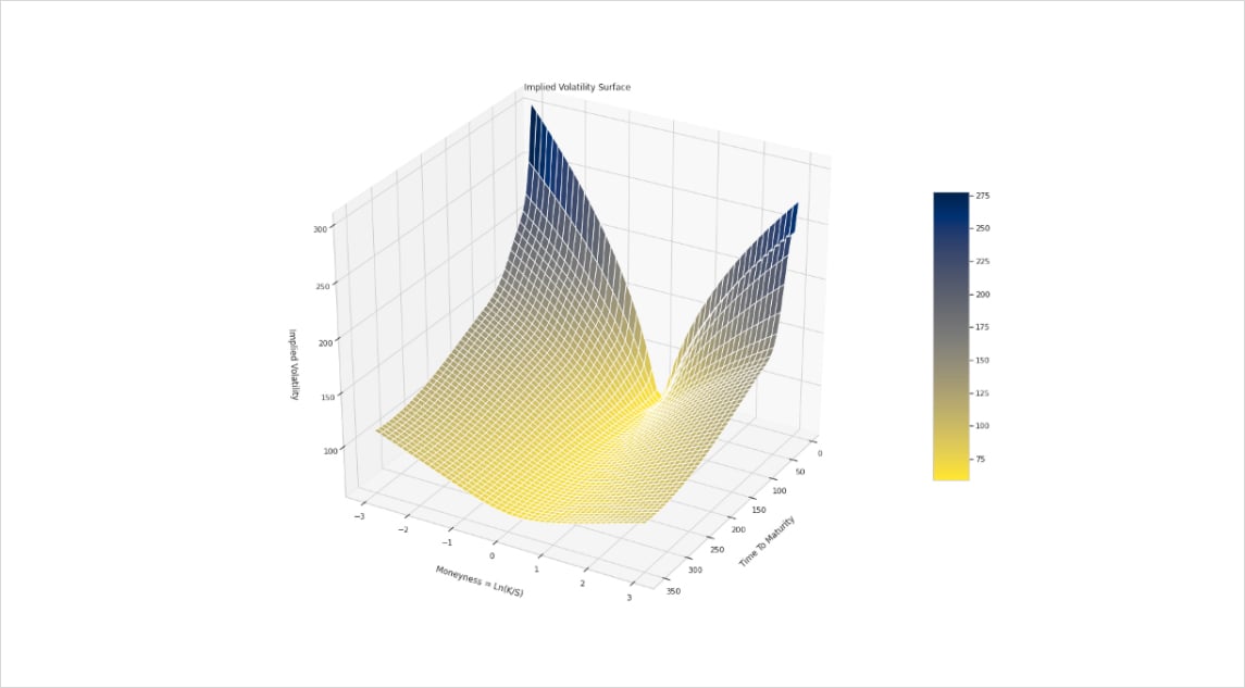
Fig 2: Implied Volatility Surface for BTC on 22/10/2021
Using this approach, we obtain for each strike K (or moneyness) and expiry T an implied volatility. So in order to price an option, we inject its implied volatility given by the surface in the black and scholes formula for better and fair pricing.
Great, we now have a way to price options using implied vols, but once we have an options book how do we manage risk around changes in the underlying, volatility or time? This is where the Greeks enter the equation.
Greeks
The Greeks, also known as risk measures, are a set of calculations you can use to measure different factors that might affect the price of an options contract. The 4 risk measures that are available on our options calculator are:
- Delta is the option price rate of change relative to every one dollar move in the underlying.
- Gamma measures the rate of changes in delta over time.
- Theta tells you how much the price of an option should decrease each day as the option nears expiration, if all other factors remain the same. This kind of price erosion over time is known as time decay.
- Vega measures the rate of change in an option’s price per one-percentage-point change in the implied volatility of the underlying.
Let’s take a rudimentary example for delta and gamma: Say we want to buy a BTC call today (07/02/2022) with a forward price of $42574, expiring on 25MAR22 with a strike price of $50000 and 62% implied volatility.
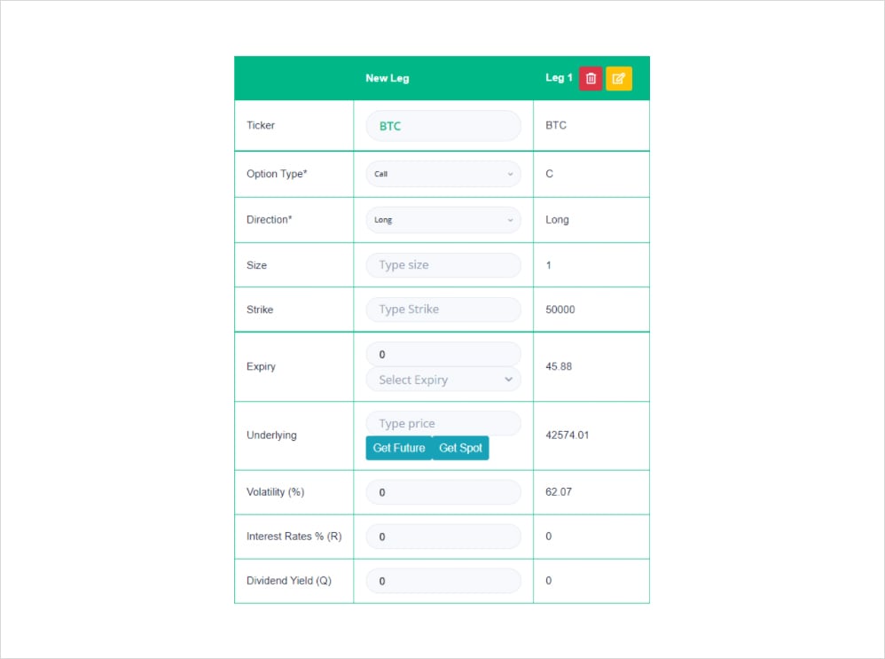
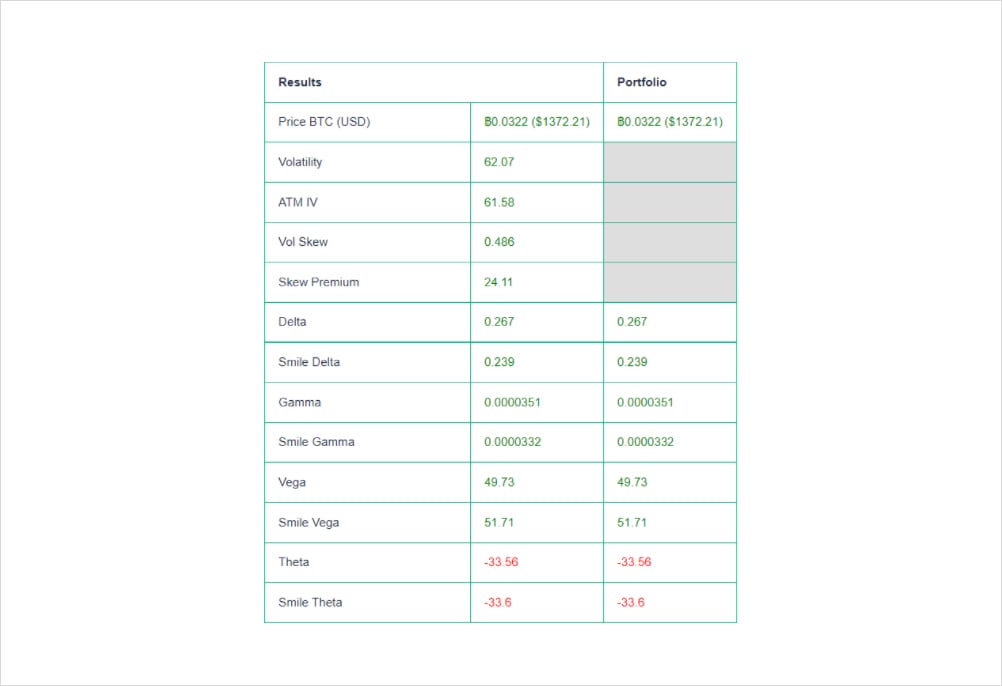
By using the Laevitas calculator we can view the premium we expect to pay 0.0322 BTC ($1372) and our risk measures. Seeing as we took a directional bet that BTC will go up and bought a call, our delta, gamma and vega are positive whereas our theta is negative since time decay will slowly eat into our position. If we focus on the “true” delta value above we expect for every $1 move in BTC our option contract will go up $0.26 (0.00000628235 BTC). Fast forward 10 days later and we hit the jackpot as the BTC price is $52k and our option is in the money (ITM). That’s a $9420 upward move in the underlying.
(Underlying USD move * delta)/Underlying Price = change in option value
- (9420 * 0.267)/42574= 0.059 BTC
Therefore we expect our option contract to go up by around 0.059 BTC (if volatility stays constant).
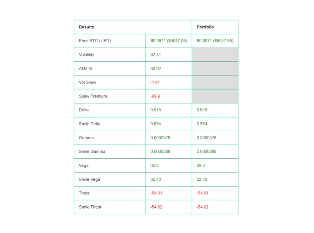
Above we see the results, our position is up by ~0.0649 BTC and the new delta is 0.618. Subsequently, since we know that gamma is the rate of change of delta over time (per $1 move in the underlying) we can easily calculate where that number came from:
Gamma * USD move = Change in delta
- 0.0000351*9420=0.33
Add to delta prior to move
- 0.267+0.33=0.597
Hopefully this example illustrates the dynamics of delta and gamma and how important these risk measures are to managing an options book. In the above image, you may also notice 2 different types of risk measures “standard” which apply B/S assumptions and smile greeks. Earlier in the article we demonstrated how implied volatility is not constant across a volatility surface, but is there an impact on our portfolio risk measures? As a matter of fact, yes and this is where the Smile Greeks intervene.
In a way, Smile Greeks are how we represent the Greeks given that the implied Volatility is not constant as opposed to the Black and Scholes assumptions:
- In the Black and Scholes world we have σ is a constant for all options. (case 1)
- Now we have σBS = σ( 𝐦, 𝛕). Where 𝐦 = Ln(K/S): the moneyness. (case 2)
Suppose that we need to calculate the delta of an option. The delta of an option is defined as the rate that measures the fluctuation of the option price when the underlying asset price changes. We have:
∆ = ∂C/∂S
Taking account that the implied volatilities are not constant across moneyness and expiry, the price of an option will be affected by a direct change in the underlying price. That’s the direct effect.
The price of an option will also be affected by the change of the implied volatility because of a change in the underlying price. That’s the indirect effect.
Schematically we have :
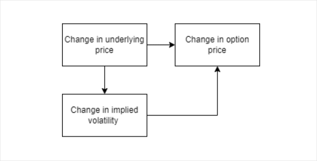
Mathematically we can express the smile delta as :
∆ = ∆BS + ∂C/∂σ ✖ ∂σ/∂S
Explicitly we have :
∆ = ∆BS + 𝝂 ✖ ∂σ/∂S
Where 𝝂 is the vega of an option. The term ∂σ/∂S represent the slope of the Implied Volatility surface with respect to the underlying price.
Using the same principle, we can get the smile greeks for each sensitivity. It gives us a better value for the Greeks while taking into account the new framework for pricing options and hedging our book.
Delta Hedging
Ideally, we hedge all risks except those we specifically want exposure to and in this case as we are trading vol, we will want to hedge the underlying. As all hedging decisions need to be made based on risk-reward, personal preference plays a big role in what would otherwise be a clean science.
The fair price of an option is drawn from the projected standard deviation of the underlying’s returns and if our Vol estimate differs from the market’s projection, we stand to generate pnl. However, it is worth noting that all outcomes are highly path dependent and therefore a seemingly correct vol estimate and adequately sized hedge may still result in unexpected outcomes. Expanding on this, if you were free to trade the underlying in any size and at no cost, the ideal play would be to continuously rebalance the underlying, that is to trade in indiscernible time increments. However, as you can only hedge discretely and by crossing the bid-offer, thereby incurring fees, we are left with the conundrum of how often and in what size? Inviting subjectivity and bias.
To further highlight this, assume you have sold USD 1,000 of Vega ATM in ETH struck ATM priced at USD 100, at 80% vol vs 70% realised. Before any costs are incurred you can expect to make USD 10,000 (Vega * (Realised – Implied)). Now add a bid-offer of USD 0.1 which must be crossed at each rebalancing and as can be seen from the table, your hedging frequency will begin to impact realised payoff despite theoretical expectations. Now factor in a not so generous spread and things become even more unappealing.
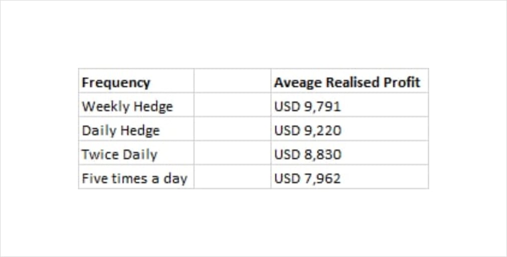
Average Profit realised when rebalancing hedges at different frequencies (In theory we would generate USD 10,000) *Reference: Euan Sinclair, Option Trading – Pricing and Volatility Strategies and Techniques
What can be done? Whilst there are several proposed solutions none of them are a silver bullet, instead they are a blend of risk aversion, economic utility, and arbitrary finger in the airness (my go to).
For illustrative purposes, these range from rebalancing at fixed time intervals e.g., end of day (right before breaking out the G&T), hedging at key levels in the underlying (targeting key psychological levels), fixed delta intervals (perhaps you want to net your deltas whenever they breach 5, 6 or however many G&Ts you’ve necked- it’s worth noting that this process in itself can get involved as the delta profile itself changes), static hedging or even a utility based framework through which you rebalance based on your level of indifference between hedging costs and exposure to unhedged risk. There’s a whole world of nuance to the art of hedging but overall, it is imperative to understand that good hedging practice is being able to reduce the most risk at least cost.
So now that we have established that I cannot simply magic away your hedging problems with an elixir, let’s delve into some examples that further showcase the futility of hedging. Only joking, we’re now going to briefly touch on price action and subjectivity.
For simplicity’s sake, let’s assume Implied vol is 10% and we choose to buy a Call struck at 1200 (dashed line), our delta hedge will lead us to sell high and buy low. Now assume 3 scenarios a) Rebalance at fixed time intervals regardless of outlook – hourly, daily etc b) Desk has a view so you rebalance based on perceived key levels c) Reassess vol bias.
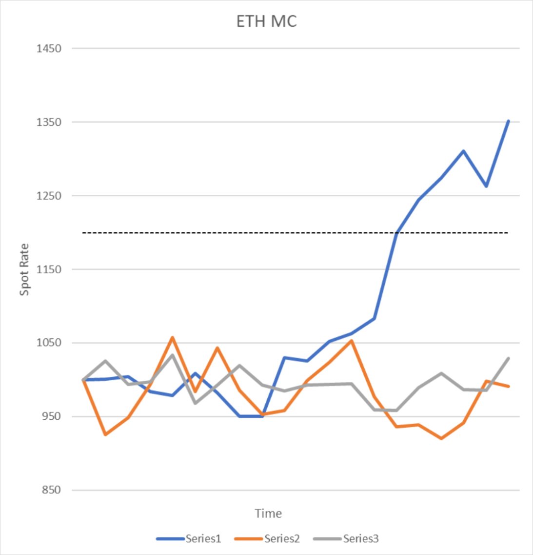
Scenario A – if we respect the set time interval hedging, we would likely fare equally on all 3 paths up until about the latter point when the blue path decides to flee the nest and ascend. Now let us tackle these paths:
Series 1 – Despite that sneaky suspicion that you may have overpaid for Vol you stick to the mandated terms and sell high and buy low at fixed intervals. This works well for you until the market suddenly lurches higher. As the market rises, you continually sell, thereby losing more and more on your hedge albeit compensated by the fact your strike is coming into sight.
Series2 & 3 – Let’s pair these paths together for now. Assuming range bound price action you would be remiss not to hedge your exposure. If price ended up being lacklustre and you didn’t have a view you would fare no worse than hedging at your given mandated hour.
Scenario B – Mystic Meg. Assuming your designated desk Tarot card reader has the foresight to draw a few lines on a chart and rightly deduces impending price action:
Series1 – Frankly there would be no reason to hedge in this scenario.
Series2 & 3 – You would want to consider your key support and resistance levels and potentially load up or clear out accordingly as it’s just a matter of time before your option expires worthless.
Scenario C – Surely there must be a substitute for crystal balls and rigid directives? An alternative would be to review your hedging vol estimate. What does this mean and how can it be implemented?
Series1 – Assume the market is trending and has clearly broken out of its range, increasing your hedging vol estimate will result in lower gamma and therefore reduced rebalancing. Thereby reducing losses relative to Scenario A while still remaining hedged.
Series2 & 3 – This sideways action would benefit from a reduced vol estimate, encouraging higher gamma and therefore delta accumulation making sure you eke out all those Sats before your option position lapses.
Note
Although Series 2 & 3 look almost indiscernible, Series2 appears to have a wider distribution. Therefore, you could be forgiven for immediately assuming Series3 has a lower vol relative to Series2 however don’t forget that vol is the magnitude in difference between daily returns, not the accumulated size of price change i.e., even though both series start and end in pretty much the same place, we are more concerned with how aggressive day to day changes are rather than whether it went further in any one direction.
If you hedge both these paths at identical fixed intervals with the same assumed vol, what do you think happens? Here’s a clue, what is the relationship between a vol estimate and gamma? That’s a teaser to make sure you return for the next write up.
Impact on Delta Hedging
On the topic of delta hedging, although different models return unique values, every trader uses their instincts and trading acumen to determine what their delta really is. One should use outputs of models as guidance to a decision, not general truth. Therefore, it is important to calculate delta based on a new framework of pricing rather than taking the BS delta at face value.
Since Delta shows how the value of an option changes as the underlying asset changes, we can take positions to create a delta-neutral portfolio. In simple words, delta hedging consists of neutralizing the extent of the option’s price compared with the underlying asset’s value. But this state is only temporary, we need to keep rebalancing our portfolio to keep up with market change and stay delta neutral.
Let’s take an example of a BTC long call position with a strike K = 30000$ where our option ends on 25 March 2022. The underlying price is equal to 38278$. 𝚫BS = 0.85
Basically we need to short 0.85 BTC to be delta neutral.
Suppose that the underlying price dropped from 38278$ to 35000$. That’s a -3278$ move.
- The change in our option price is : -3278 * 0.85 = -2786 $
- The gain we did by shorting 0.85 BTC : (38278 – 35000) * 0.85 = + 2786 $
- Our portfolio change = -2786 + 2786 = 0
By keeping our portfolio delta neutral we keep the value of our portfolio intact regardless of underlying mouvements. But what if we use the smile delta as our trusty indicator for hedging?
The chart below depicts the difference between the BS delta and Smile delta for that option:
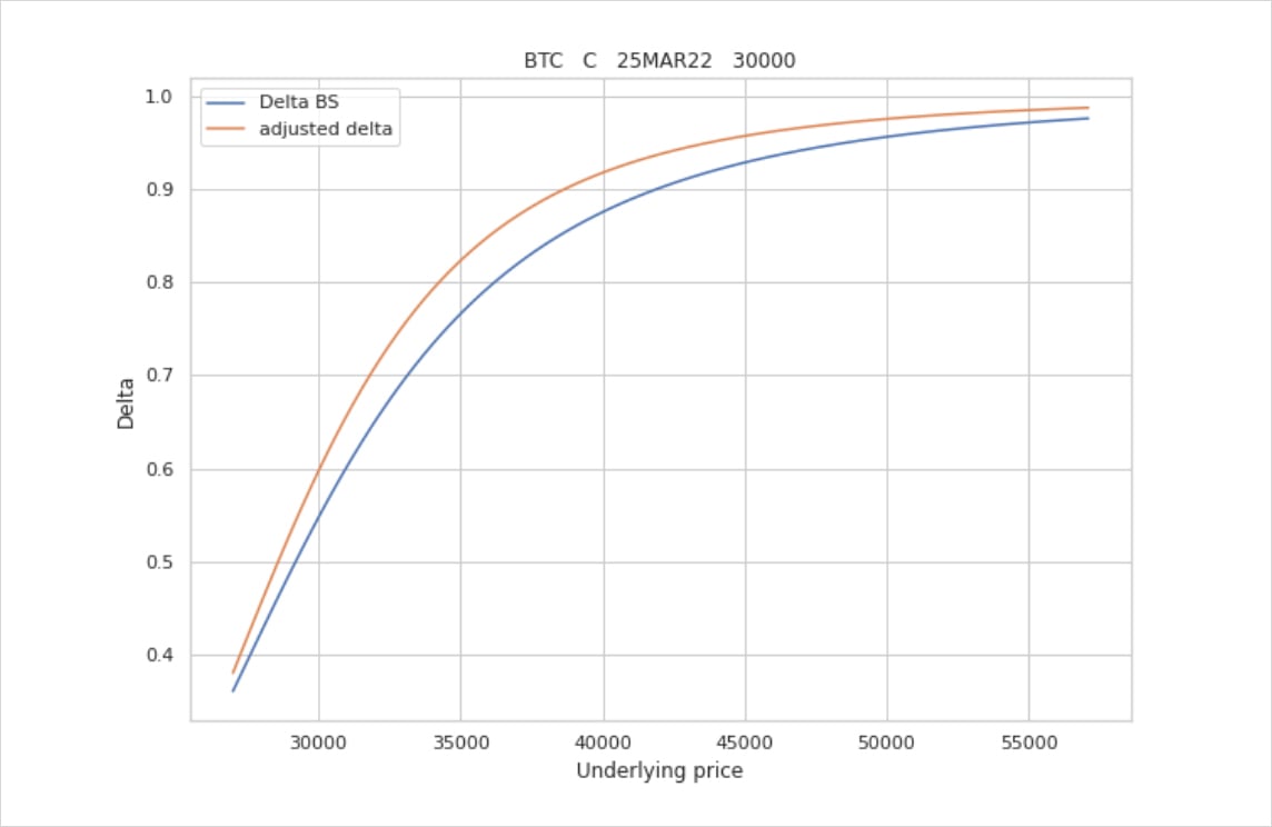
As we can see above, the adjusted delta is higher than the theoretical delta given by B-S assumptions. Which actually means that we should sell even more units of the underlying asset in order to stay delta neutral.
Back to our example, the Smile delta is equal to 0.9 as opposed to Black and Scholes delta which is around 0.85.
The drop of the option value should be : -3278 * 0.9 = -2950.2$
That‘s -164.2$ more compared to the drop of the option price if we used Black and Scholes theoretical delta and that’s for a single option!
Now imagine if we have a position where the size is over hundreds of contracts. This is where the impact of delta hedging according to different models comes into effect. If you’re managing a large options book, building the right framework and using the correct assumptions for managing risk is crucial. This is our goal at Laevitas in building a robust options pricing tool, the end game is to allow users to manage their options risk using different models, assumptions and market conditions. We’re excited to share more info alongside our upcoming updates!
Conclusion
To conclude, I hope this high level explanation of the volatility surface and how it impacts hedging around an options book, helped clarify some nuances around the different models which exist today in terms of calculating risk metrics and managing risk. For further reading on this topic, this paper by Emanuel Derman is a great resource. We welcome any feedback on the above and the options calculator, please feel free to reach out on our Discord.