

Expected move on Deribit
It is now possible to see the expected move on the Deribit option chain. As this calculation and visual is a new addition to Deribit, many users may not be familiar with it yet, so we will first explain where to find it in the UI, and then explain what it is in more detail.
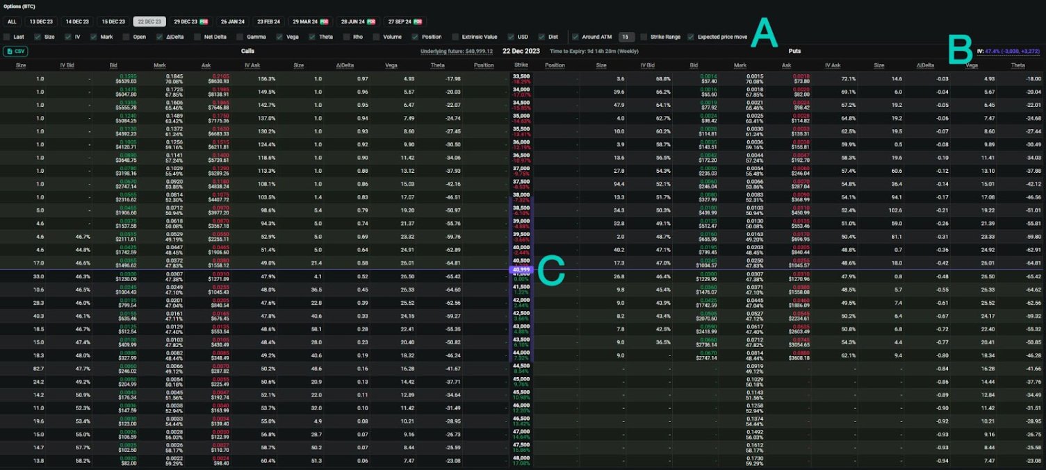
Point A shows where the expected move can be enabled or disabled.
Each expiry date has a different expected move, calculated using the at-the-money (ATM) implied volatility. The implied volatility used, as well as the size of the expected move up or down, can be seen in the top right of the header for each expiry date in the option chain (point B).
At point C, the current underlying price is highlighted in the Strike column, in the centre of the option chain, with a horizontal line indicating which strikes the underlying price is currently between. On the left and right sides of the Strike column, the expected move is shown with the shaded area.
What is the ‘expected move’?
You may hear some option traders talk about the ‘expected move’ of a particular asset. This phrase refers to the expected size of price movements the asset may have by a certain date. This could be in the next day, the next week, or even the next year.
For example, if we are looking at an underlying asset with a current price of $50 and an expected daily move of +/- $2, this means that in 24 hours the price is most likely to be between $48 and $52, according to the expected move.
Or, if we are looking at an underlying asset with a current price of $90 and an expected move for the next 7 days of +/- $8, this means that in 7 days the price is most likely to be between $82 and $98.
‘Most likely’ is quite a vague term here, but we can be more specific.
Firstly, we should be clear about where this figure is coming from. The expected move figure is calculated using the current price of ATM options on that asset. So when we say the “expected move for the next 7 days is +/- $8”, what we are really saying is the current price of the ATM options that expire in 7 days are implying that the price is most likely to be between $82 and $98 when those options expire.
Next, we can give more detail on what we mean by ‘most likely’.
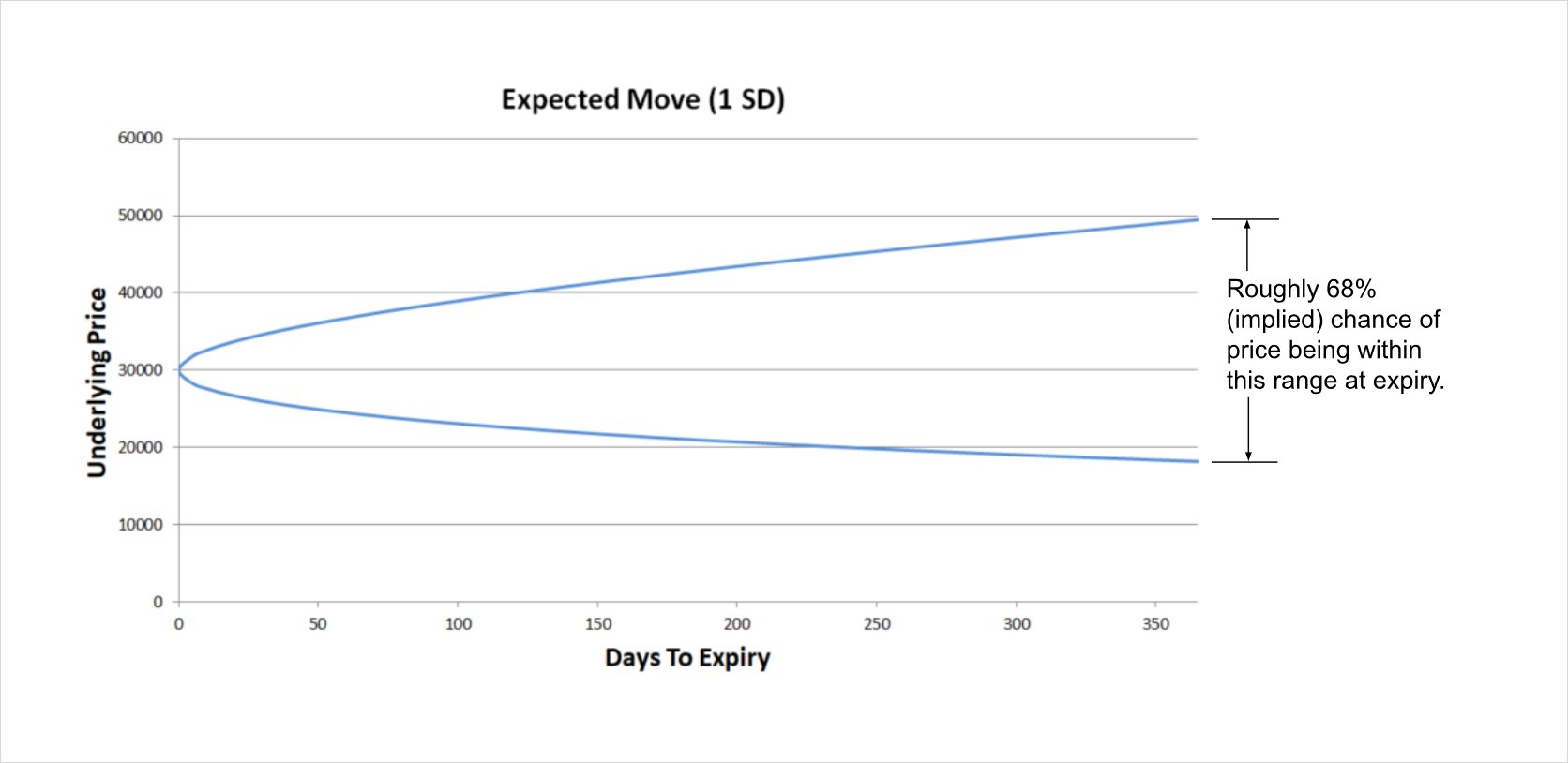
The ‘expected move’ as it’s often called can be thought of in mathematical terms as the estimated one standard deviation move. That is, the price range which is expected to contain the future price roughly 68% of the time.
In this image, the expected move has been calculated for up to one year, assuming an underlying price of $30,000 and an implied volatility of 50%.
A standard deviation is a measure of how close the individual values typically are to the mean of a distribution. In this case we are talking about the distribution of the possible future prices of some asset, in relation to the current price. We are using the ATM implied volatility as our estimate for the standard deviation of that distribution.
This chart shows the one standard deviation expected move depending on how much time is left until expiry, and for various levels of implied volatility.
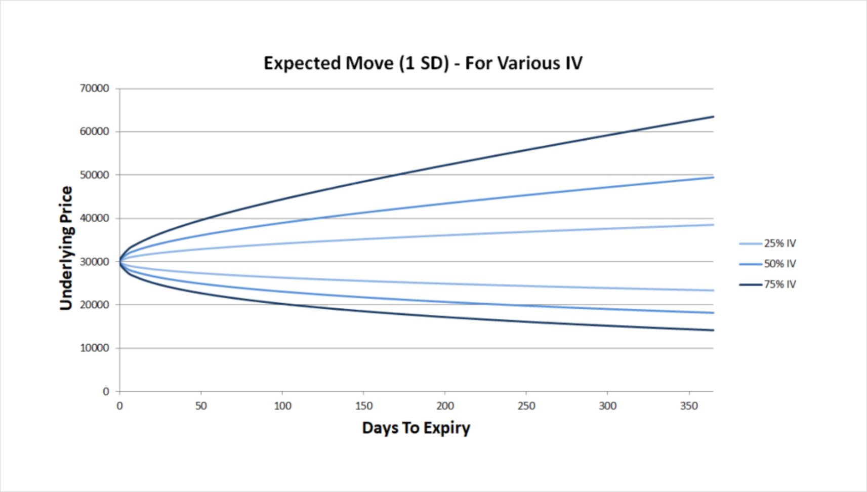
The higher the implied volatility, the less confident the market is about the future price of the asset. This leads to larger expected moves, as the implied range of possible future prices is larger. Conversely, the lower the implied volatility, the more confident the market is about the future price of the asset. This leads to smaller expected moves, as the implied range of possible future prices is smaller.
What expected moves can and can’t tell us
It’s worth taking the time to point out that when we’re talking about the probability of where the underlying price could move to in this context, we are talking solely about the market’s view, as expressed through the price of options. We are talking about implied probabilities then, and not about the actual probabilities of certain prices being reached.
Expected moves can tell us something about the market’s view of the distribution of possible prices, but it can’t tell us how accurate this view will prove to be. In other words, we use implied volatility (option prices) for expected move calculations, which allows us to calculate the market’s expected move, but the market could be wrong.
We are also assuming that the future price is lognormally distributed, which it may not be. However, despite these limitations, the expected move is a useful, simple statistic, as it shows at a glance what the market’s current view is on how far the underlying price is likely to move in future.
Calculating the expected move
To calculate the one standard deviation expected move we use the following formulas:
The expected range low is given by:
Underlying Price / (exp(ATM_Vol * sqrt (T)))
The expected range high is given by:
Underlying Price * (exp(ATM_Vol * sqrt (T)))
To get the size of the up and down move we can then simply subtract the underlying price, such that:
Down Move = (Underlying Price / (exp(ATM_Vol * sqrt (T)))) – Underlying Price
Up Move = (Underlying Price * (exp(ATM_Vol * sqrt (T)))) – Underlying Price
Where:
Underlying Price = The underlying price. On Deribit this will be the price of a futures contract.
exp = The exponential function
ATM_Vol = The at-the-money implied volatility. (Linear interpolation is used if the underlying price is between two strikes)
sqrt = The square root function
T = Time to expiry in years
Example calculation
If we have the following parameters:
Underlying Price: $30,000
ATM_Vol: 40%
Time to expiry: 30 days
Then we can calculate the expected down move as:
= (30000 / (exp(0.4 * sqrt (30/365)))) – 30000
= (30000 / 1.121510498) – 30000
= $3,250.36
And the expected up move as:
= (30000 * (exp(0.4 * sqrt (30/365)))) – 30000
= (30000 * 1.121510498) – 30000
= $3,645.31
This would mean that the ATM IV is implying that there is roughly a 68% chance that the price in 30 days will be between $26,749.64 and $33,645.31.
Why calculate up and down moves separately?
If you have seen expected move values before on other option platforms, you may have seen them stated as a single plus/minus figure (e.g. +/- $50). This makes it simpler to display as the expected move is symmetrical, and for low time frames like daily moves, or for low volatility environments, this can be sufficient. With higher volatilities though (larger standard deviations), and/or a longer time to expiry, it becomes necessary to consider the likely size of the move in each direction separately.
To illustrate why, let’s assume we have some asset with a current price of $100, and an ATM IV of 30% with 25 days to expiry.
The symmetrical expected move, which assumes the distribution of possible future prices are normally distributed, would be stated as +/- $7.85. (This is calculated as Underlying Price * ATM_Vol * sqrt(T))
Assuming that future prices are lognormally distributed instead, and therefore calculating the up and down move separately, would give us +$8.17, -$7.55.
In this first example then, both calculations are relatively close to each other, and both seem like plausible estimates.
However, let’s now assume the asset is still priced at $100, but now has an ATM IV of 90%, and a time to expiry of 500 days.
Our lognormal calculations give us an expected move of +$186.73, -$65.12. This results in an expected price range of $34.88 to $286.73. This is a very wide range, but with such high volatility, and a long time until expiry, having a wide range of possible future prices makes sense.
The symmetrical calculation gives us +/- $105.34. This results in an expected price range of -$5.34 to $205.34. It should be clear to all that this is not realistic, and that this is therefore not a very useful statistic. Assuming that possible future prices are normally distributed gives the possibility of negative asset prices. Assuming instead that future prices are lognormally distributed, eliminates the possibility of negative asset prices, and gives us a much more realistic model.
It is unlikely to be the case that the distribution of the possible prices of an asset at some point in the future is precisely lognormally distributed. However, we can assume that using a lognormal distribution is more accurate than using a normal distribution. It is for this reason that we use the lognormal distribution, which is not symmetrical, and therefore we have to calculate the up and down move separately.
Using the expected move
The values and highlighting for expected moves in the Deribit option chain give traders a quick way to visualise likely possible moves for the underlying asset for each expiry date. This will particularly aid traders who like to trade options based on where the strike price sits, relative to likely moves in the underlying price.
Expected moves do not encompass all possible outcomes though, as they are only showing a one standard deviation expected range, which even if accurate, would only contain the price roughly 68% of the time. So while still useful, it is important for traders to recognize that expected moves are merely the market’s view on ‘likely’ moves, as expressed through option prices. The underlying price at expiry will not always land in the expected range, and they should not be relied upon exclusively.