

The two statistics Implied Volatility Rank (a.k.a. IV Rank, or IVR) and Implied Volatility Percentile (a.k.a. IV Percentile, or IVP) both measure how the current level of implied volatility (IV) compares to the historical range of values for IV. It’s possible to calculate these statistics for any period of time, but it’s most common to use the range of values over the previous year.
IVR ranks the current IV against the historical range of IV over the last year, and IVP shows what percentage of time the IV was lower than the current level over the last year. Both measures give a value between 0 and 100. We’ll get into how each differs soon, but for both IVR and IVP, a value of 0 means IV is very low compared to normal, and a value of 100 means IV is very high compared to normal. With ‘normal’ here simply meaning the range of values over the last year.
As IV tells us how cheap or expensive options are, both IVR and IVP can be used to gauge how cheap or expensive options currently are, compared to typical values for each underlying.
IVR and IVP give context to IV
IV allows for better price comparison between different options. This is because it takes into account the factors that affect how much an option is worth, like time and moneyness*. This allows each option price to be stated as an annualised volatility figure.
*Moneyness = where the strike price is relative to the current underlying price.
IVR and IVP give further context to this by allowing for better comparison to historical norms for the underlying.
For example, even if you have traded options before, if you were new to trading cryptocurrency options specifically, you might not be familiar with what typical implied volatility figures are for bitcoin or ethereum. If the IV for bitcoin is sitting at 45%, is that high or low? 45% IV would be high for something like US Equity index the S&P 500, but it would have been low for the meme stocks like Gamestop or AMC that became popular amongst retail option traders in 2021. We need to give some context to the IV figure.
IVR and IVP give us this context by comparing the current IV for an asset to historical values of IV for that same asset. Each statistic simplifies this comparison down to a single value between 0 and 100, with each one telling us something slightly different.
Calculation methods
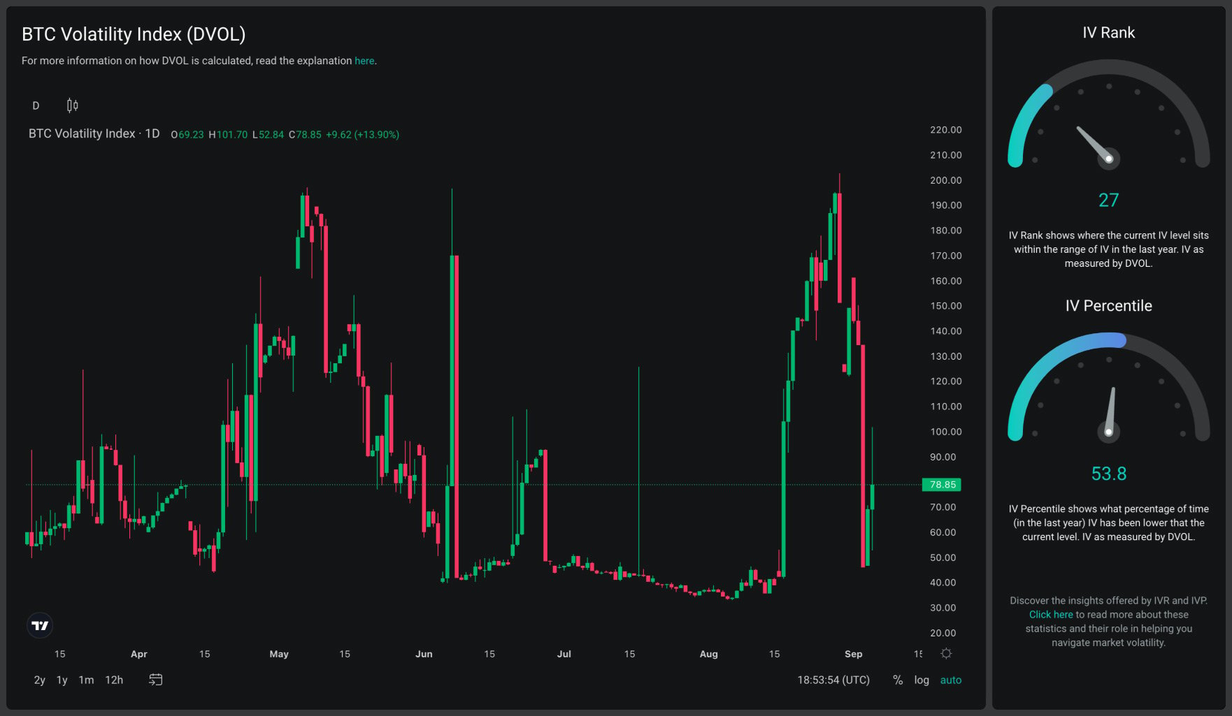
Thankfully the calculations are relatively simple. All we need is the historical data for IV, and for that we will use the DVOL index data.
Information on DVOL can be found here.
IVR tells us how far into the historical range of IV the current value of IV is, and is calculated as:
(Current IV – IV Low) / (IV High – IV Low) * 100
Where:
Current IV = the current level of implied volatility.
IV Low = the lowest value that implied volatility has been for the underlying in the last year.
IV High = the highest value that implied volatility has been for the underlying in the last year.
(All as measured by DVOL)
IVP tells us what percentage of the time IV has been below the current value of IV, and is calculated as:
Periods Lower / Total Periods * 100
Where:
Periods Lower = the number of periods in the last year that implied volatility has been lower than the current level.
Total Periods = the total number of periods in the last year. E.g. if the period is 1 day, the total number of periods is 365.
The only data that is required to calculate both of these statistics is the last year of historical data for the DVOL index.
Why show both IVR and IVP?
Both statistics are showing a different version of the same thing, as they both show how current IV compares to IV over the last year for the underlying we are looking at. However, it is still useful to see both due to the differences in how they behave with certain data.
IVR is more sensitive to outlier values. A single occurrence of dramatically higher IV could lead to relatively lower values of IVR for a long time, until that single data point has fallen out of the comparison period (usually one year). IVP does not suffer from this because it’s not looking at the full range of values, and only measures how much time is spent below the current level of IV, so a single day’s IV value only counts 1/365th towards the IVP value.
IVP can be overly sensitive to small changes in IV though, depending on where current IV is relative to the distribution of the previous values. Whereas IVR deals with the scale of moves in IV more consistently. A small change in IV will typically mean a small change in IVR.
An example of how IVR and IVP can differ
Imagine the current IV is 60, and we have the following 10 historical readings for IV.
[100, 50, 70, 59, 50, 50, 50, 50, 50, 50]
IVR here would give us a reading of just 20, because the value of 60 sits 20% of the way into the range of 50 to 100.
(Current IV – IV Low) / (IV High – IV Low) * 100
= (60 – 50) / (100 – 50) * 100
= 20
This makes it seem like IV is quite low compared to usual. However, the current level of 60 is higher than most of the previous readings.
Let’s see if IVP gives us any more information. IVP is calculated as:
Periods Lower / Total Periods * 100
= 8 / 10 * 100
= 80
A very different impression is given by the IVP here. It’s telling us that the IV has been lower than the current value of 60 for 80% of the time.
Together, these two statistics tell us that although IV has been quite a bit higher than the current level of 60 at some point in the past, it has spent the majority (80%) of the time below this level.
Usually, the two statistics won’t be as far apart as they were in this contrived example, and they will typically be telling us a similar story. For example, if they are both over 90, we can be confident that IV is higher than normal. If they are both below 10, we can be confident that IV is lower than normal. If they do ever diverge though, we can look at the DVOL chart to see why.
Continuing with this example
Let’s say that we move forward one time period. We are still only going to use the 10 previous readings for comparison, so our historical values are now:
[50, 70, 59, 50, 50, 50, 50, 50, 50, 60]
Note that the previous high value of 100 has dropped out of the dataset.
Let’s also assume that our current reading for IV is 61. This is just one point higher than our previous value of 60, so IV has barely moved. How has this affected our readings for IVR and IVP?
IVR = (61 – 50) / (70 – 50) * 100 = 55
IVP = = 9 / 10 * 100 = 90
The IVR has moved from 20 to 55, and the IVP has moved from 80 to 90. IV did increase very slightly from 60 to 61, so it’s not surprising to see these two statistics increase. However, we can now see what a dramatic impact that one data point that dropped out of the dataset was having on the IVR. The range changed from 50-100 to 50-70. So despite the relatively small increase in IV, the IVR increased dramatically, whereas the IVP increased by a much smaller amount.
Finally, imagine we move forward one more time period, so our historical values are now:
[70, 59, 50, 50, 50, 50, 50, 50, 60, 61]
Let’s assume that our current reading for IV is now 58. This is just three points lower than our previous value of 61. How has this affected our readings for IVR and IVP?
IVR = (58 – 50) / (70 -50) * 100 = 40
IVP = = 6 / 10 * 100 = 60
IV has decreased, so it’s not surprising to see both values decrease. IVR moved from 55 to 40 (a decrease of 15), but IVP moved from 90 to 60 (a decrease of 30). This move in IVP would seem to exaggerate the relatively small move of 3 points in IV. This occurs because an increasing number of the data points are close to the current IV level. So as the current IV moves either side of this cluster of values, there is a larger percentage of the values that become either over or under the current level.
With this example, we’ve covered how to calculate each statistic, as well as what circumstances can lead to oversized moves in each. We have seen that IVR can change dramatically solely because one extreme data point has fallen out of the comparison period. And we have seen that IVP can change dramatically even when IV has only changed by a relatively small amount. This occurs when a lot of the previous data points are clustered close to the current IV.
So, just long relatively low IV, and short relatively high IV, right?
Well, although volatility is mean reverting over the long term, it tends to cluster in the short term. This means it can maintain extreme values over the short term. Just because IV is very low, with IVR and IVP both showing values of less than 5, doesn’t mean that IV won’t continue to be low for several weeks, or even months.
It’s also worth bearing in mind that even if IVR and IVP are both sitting at the maximum value of 100, that doesn’t mean volatility can’t increase even further. The reading of 100 simply means that IV is the highest it’s been in the measurement period (usually 1 year). However, it can still increase further, setting a new record high, and keeping the IVR and IVP values pinned at 100 until IV finally falls away from the new high.
Similarly, when IVR and IVP are both at the minimum value of 0, volatility can still decrease further.
So, although extreme readings may tilt the odds in favour of mean reversion, there is no guarantee.