

In this article, Amberdata will take you through a larger analysis of BTC Options.
Options are gaining more and more importance for a Crypto Trader. This analysis takes you through data starting from 2019 until now – Overall development and how you might be able to take advantage of them.
Table of Contents:
> Forward
> Introduction
> ATM Term Structure
> Spot/Vol. Dynamics
> VRP
> Volume and Open Interest
Backtesting Strategies:
> Harvesting BTC’s Risk-Reversal Premium
> Systematic Volatility Trading
Forward
The nascent crypto asset class is only 15-years old and has presented investors with unique challenges and opportunities with respect to valuation.
Deribit traded its first BTC options in November 2016, making the crypto space even richer with opportunities by layering-in tradable volatility.
We explore big questions that remain in crypto volatility by dissecting the volatility surface and its associated regimes.
Although the crypto volatility space being new brings a unique set of challenges, it also enables astute investors to become skilled and competitive in the space. No one has a substantial head-start, so to speak.
We are committed to being pioneers in crypto volatility analytics and to helping our customers find moneymaking opportunities. As such, Amberdata Derivatives will make all the following analysis available to our customers.
Thank you for your continued trust and confidence in Amberdata.
Introduction
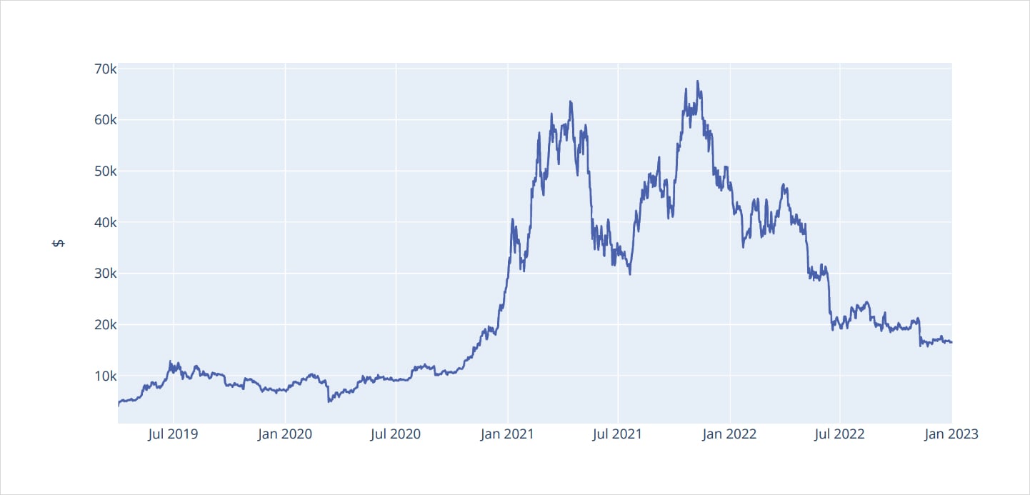
Bitcoin Spot Prices
When Deribit first launched its exchange there wasn’t an ERC-20 standard built on Ethereum yet, nor was there a reliable stablecoin market.
This led to the creation of an “inverse” options and futures exchange, meaning that BTC options and futures are collateralized by BTC itself and cash-settlement also occurs in BTC (AKA “coin”).
From 2019 through 2022, we’ve seen a lot of diff erent regimes and investment cycles around BTC and the associated options trading on Deribit.
2019: This was the tail-end of the 2018 bear market. The spot market was mostly quiet and a lot of enthusiasm for BTC investing had faded away. BTC hit its bear market low in December 2018, then prices consolidated for most of the fi rst half of 2019. Only later in the year did BTC spot prices rally to $10k, a major level of spot traders.
2020: In 2020 we had two signifi cant events. First March 2020 had the Covid meltdown. This was a scary sell-off in spot prices that caused a drop of 50%, accompanied by volatility which exploded higher. Prices then consolidated back around the $10k level for much of the year. Volatility hit extreme lows in the summer of 2020 only to end the year with a massive bull-market breakout.
2021: That year started with a bullish-breakout. In January of 2021, we saw extreme positioning in the options market as BTC quickly slid through new alltime highs day after day. Extreme positioning then leaked into the futures basis during April 2021, only to completely collapse in May 2021 after a nasty market correction.
2022: That year can be categorized into a bear market year as spot prices retraced from their November 2021 peak. The fundamental picture in crypto became bleak and quickly escalated as LUNA imploded, 3AC ran into trouble and darling exchange FTX turned out to be fraudulent, broke and actively traded against its own clients (Think 3AC’s book).
All taken together, we have a subject dataset with a multitude of spot cycles and associated volatility regimes.
Our analysis starts on April 1st 2019 and concludes on December 31st, 2022.
ATM Term Structure
ATM Constant Volatility
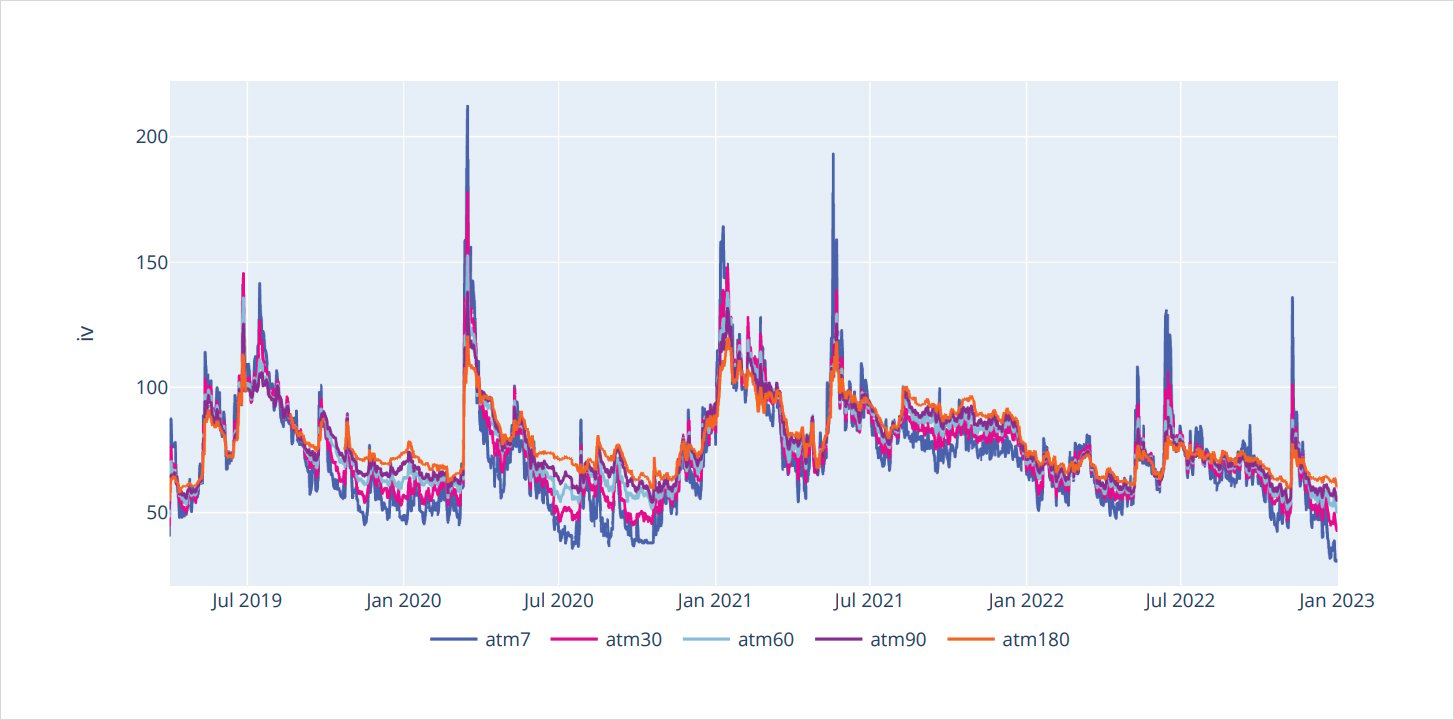

The term structure is one of the most signifi cant measurements of the volatility surface. The term structure is essentially the “spine” of the volatility surface and has signifi cant importance because it deals with ATM (at-the-money) options, which have the most extrinsic value and “optionality”, so to speak.
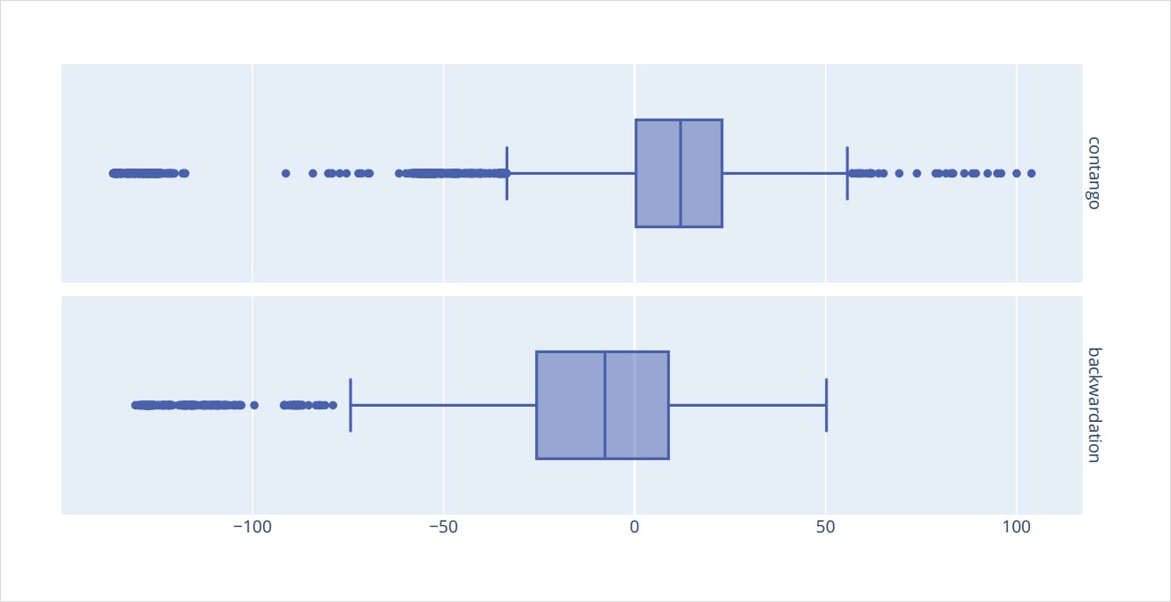
Using our subject data set, we can see that the term structure is in Contango almost 77.5% of the time and rarely in Backwardation.
Backwardation occurs in reaction to volatility “shocks” such as March 2020.
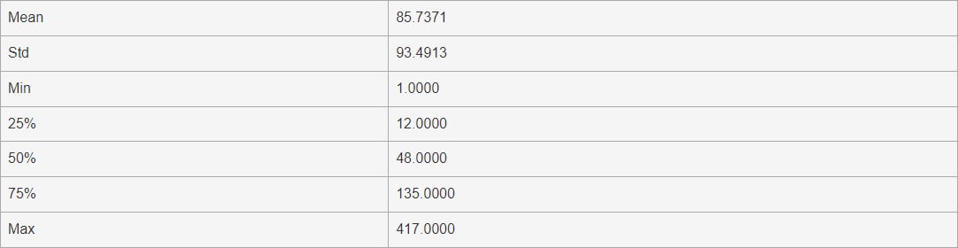
Consecutive hours of backwardated term structure
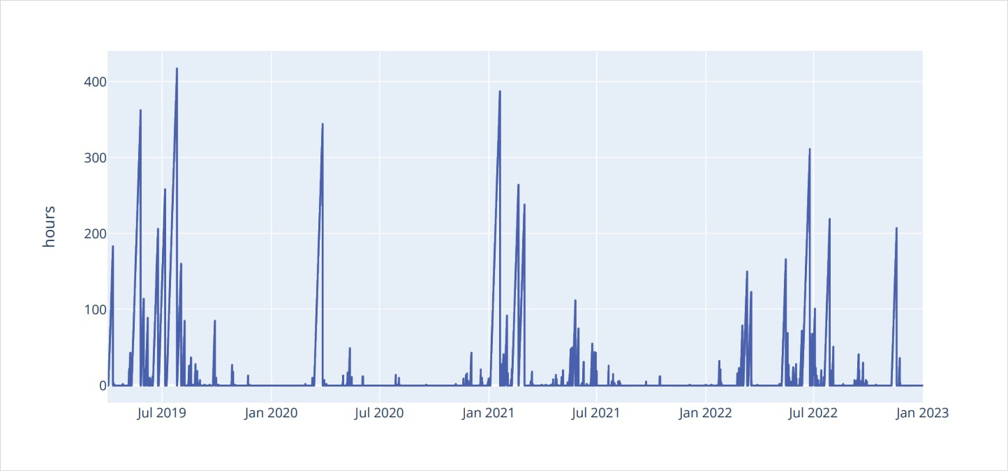
Since Backwardation is the abnormal state of affairs, we have calculated the time spent in Backwardation. Volatility traders can use the “time-to-live” (TTL) measurements to estimate when vol bets should revert into Contango.
The mean TTL of Backwardation in the Amberdata dataset is around 85 hours.
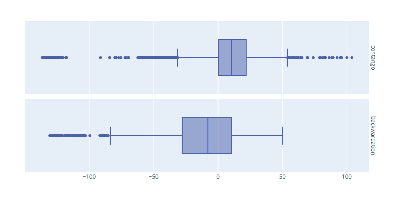
Richness (+premium/-discount) of term structure (+ backwardation/-Contango)
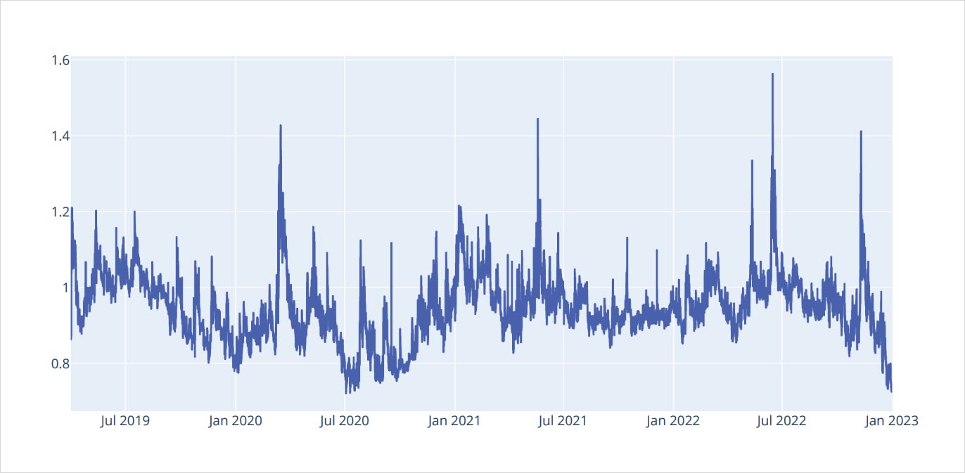
Another important measurement of the term structure is the relative “level” of the Contango or Backwardation shape.
A reading of 1.00 would be a perfectly fl at term structure – as measured by our method – while readings below/above represent Contango/Backwardation respectively.
Using the term structure levels enables us to quantify how extended the term structure pricing currently is, at any point in time.
Notice that March 2020, May 2021, June 2022 and November 2022, all represent “vol shocks” that blindsided the market but peaked around the 1.45 level.
Richness of term structure box plot
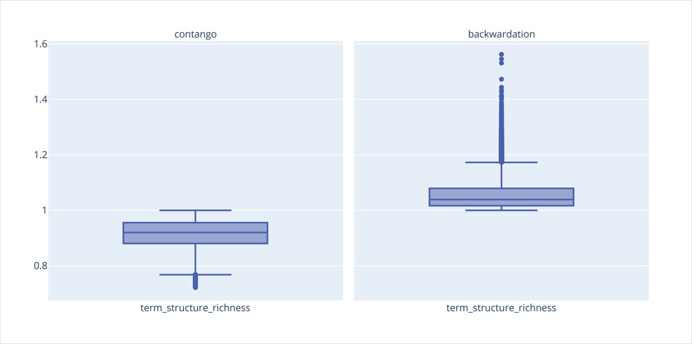
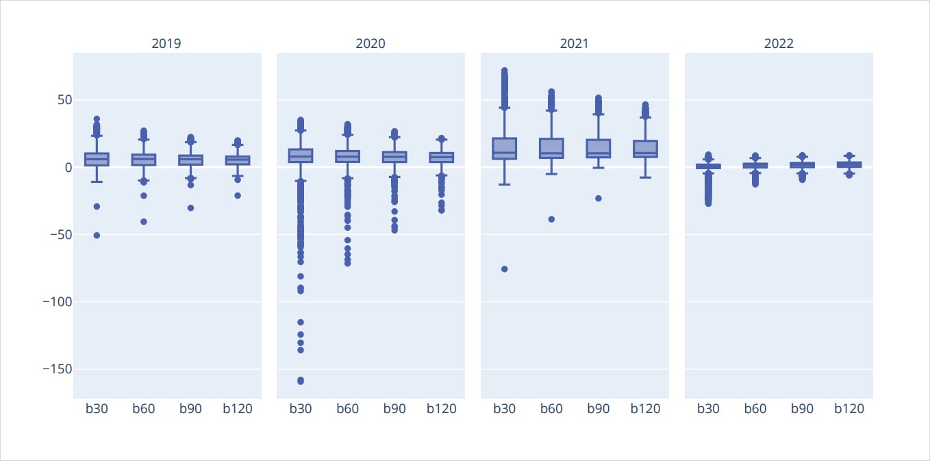
We can further investigate the term structure “levels” by separating the readings between two subsets (Contango/Backwardation) and then applying percentile distribution analysis.
We can see that the mean Contango reading is about 0.93, while the mean Backwardation reading is about 1.03.
Spot/Vol. Dynamics
Rolling 7 days linear regression of log returns Spot/atm30
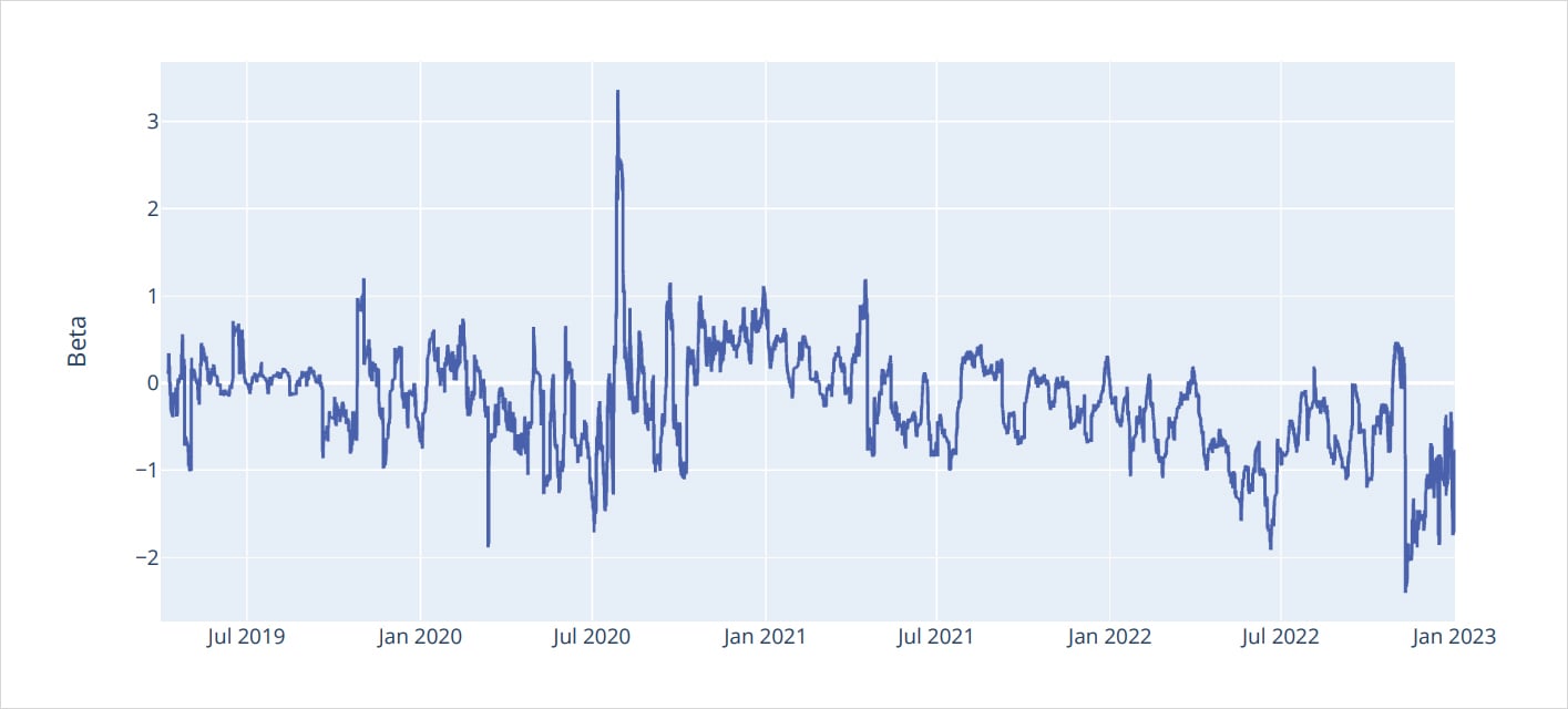
Taking the previous analysis one step further, we can now investigate how spot markets affect ATM volatility. We compare spot and 30-day ATM volatility (customers can easily pass different parameters for analysis) both on a 7-day rolling window above and as a scatter plot using hourly data, below.
Correlations log returns Spot/atm30
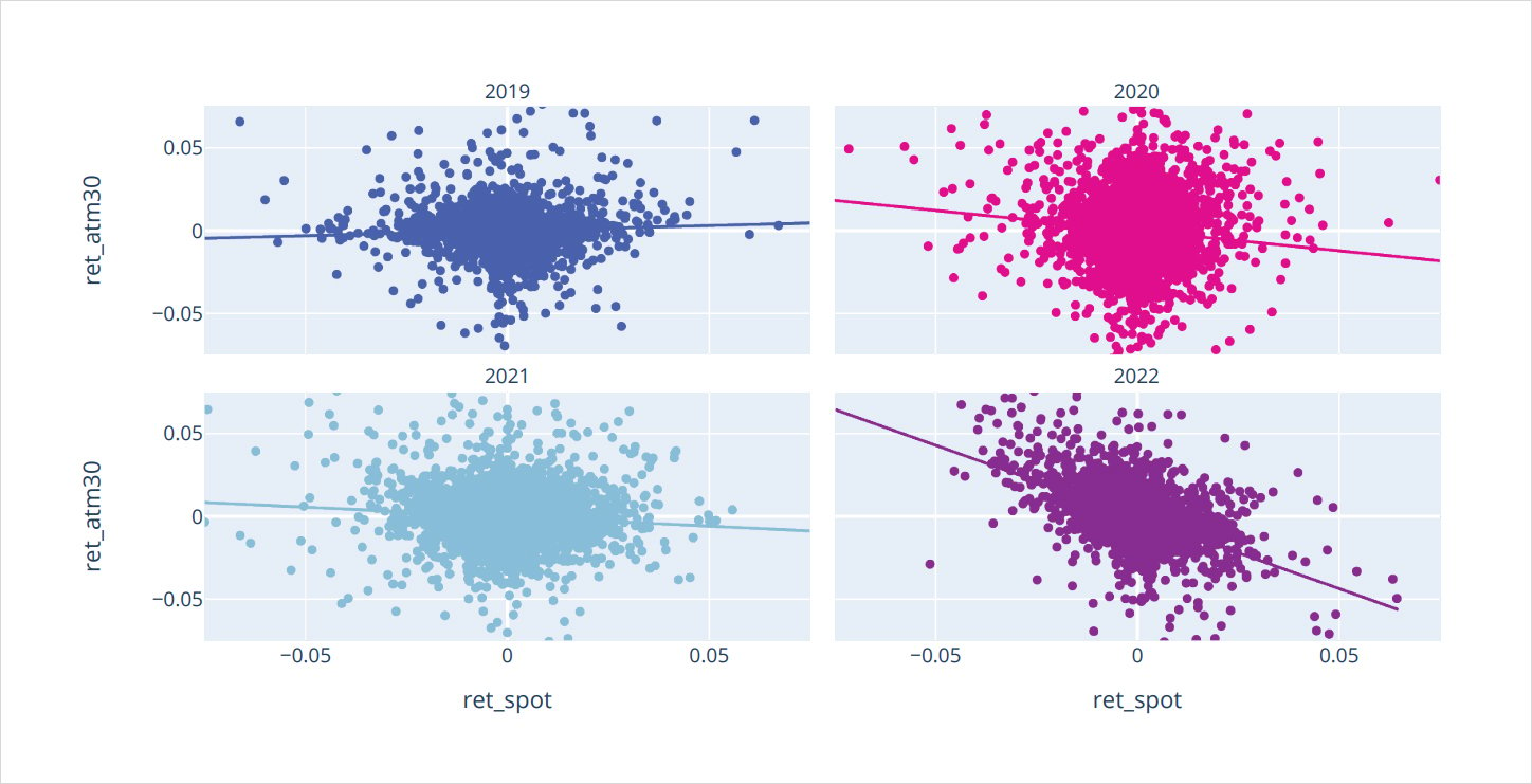
2022 stands out as a regime-changing year. We can see a much more negative scatter plot slope and a “tighter” range of readings.
On the rolling plot, we can also notice deeply negative and persistent readings of the beta values.
One of the big questions in crypto vol is whether this shift is cyclical (temporary) or structural (persistent).
In traditional markets, equity spot/vol regimes will be negative (like we see in 2022 for BTC) but commodities often display a positive relationship, as production & demand shocks affect the commodity volatility space in a different way.
While we described the ATM term structure as the “spine” of the volatility surface, the wings would be the OTM (out-of-themoney) options. Specifically, we analyze the Δ25 OTM options. The relationship between the Δ25-Call implied volatility (minus) the Δ25-Put implied volatility would be the RR-Skew (RiskReversal Skew).
Skew 30 box plot
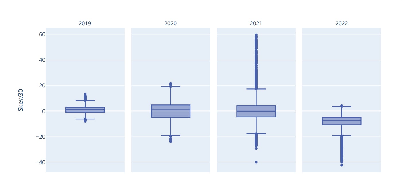
We can see two big trends when the RR-Skew is grouped and analyzed by different year buckets.
First, although 2020 and 2021 had similar variance in the term structure analysis, the RR-Skew was much more muted in 2020 than in 2021.
2021 stands out as a clear outlier in terms of overall RR-Skew range.
Secondly, the total range of RR-Skew for 2019, 2020, and 2021 is loosely symmetrical. A clear outlier to this trend is 2022, where the RR-Skew is decidedly negative and nearly never positive.
ATM30/Skew30 scatter plot per year and quarter
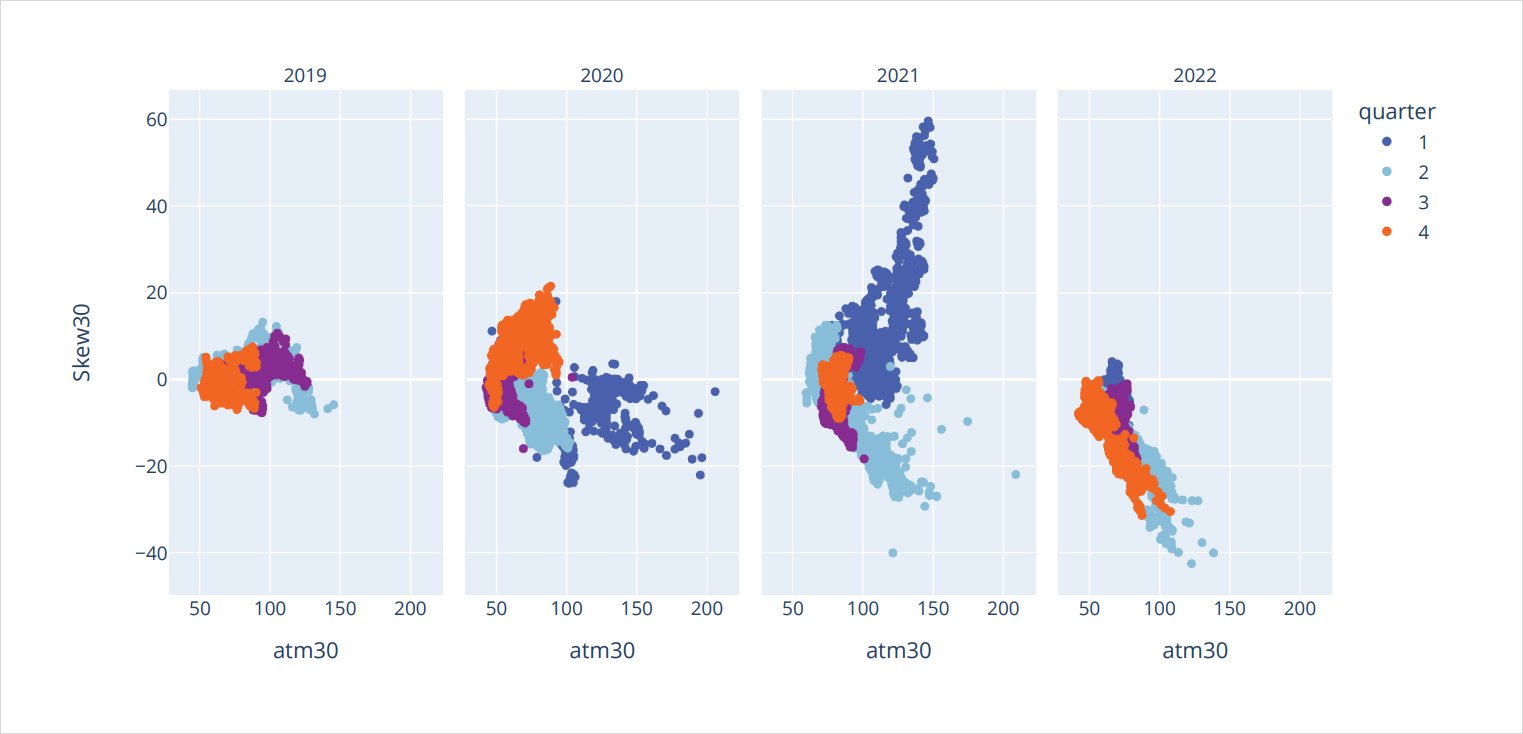
Layering the relationship between 30-day ATM implied volatility and the 30-day RR-Skew, we can see that 2021 and 2022 have two completely inverse relationships. 2021 is marked by upside momentum – especially true for Q1 2021. As implied volatility increased the RR-Skew became more and more positive.
2022 saw the opposite, especially pronounced in Q2 and Q4.
As implied volatility came into the market, the RRSkew became more negative.
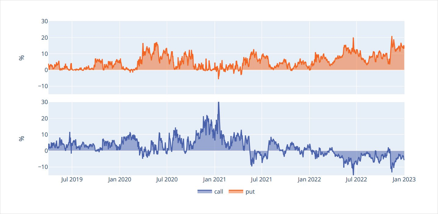
25Δ vs ATM Ratio Normalized constant 30 days
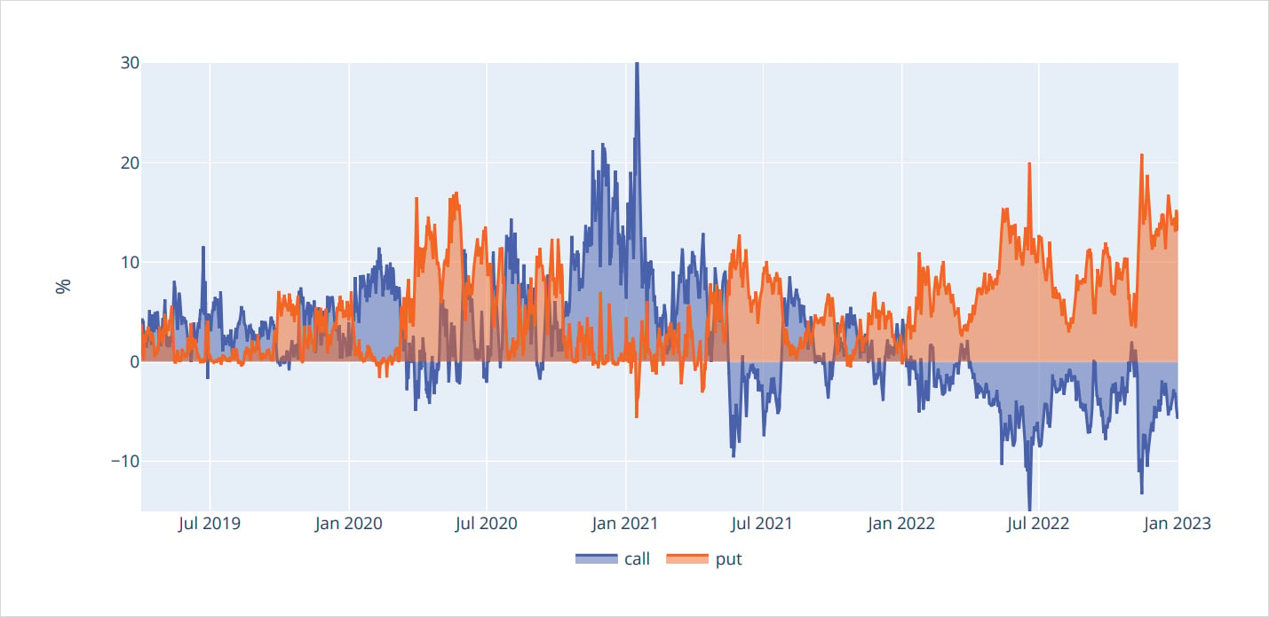
25Δ vs ATM Ratio Normalized constant 30 days
If we isolate the Δ25 Call/Put wings and ratio them by ATM volatility, we can see that call wings began to persistently trade at a discount to ATM IV (by nearly 10%) – a phenomenon similar to equity index volatility – starting in July 2021.
Puts have never traded at a discount to ATM volatility, but in the bullish market of Jan 2021, we can see Δ25 Put IV traded on par with ATM IV. This type of volatility pricing is enticing for 1×2 and put ratio spreads, which allow you to buy 2 OTM options with nearly no IV premium to the ATM option you’re selling.
VRP
Atm-rv 30 day (ATM SHIFTED)
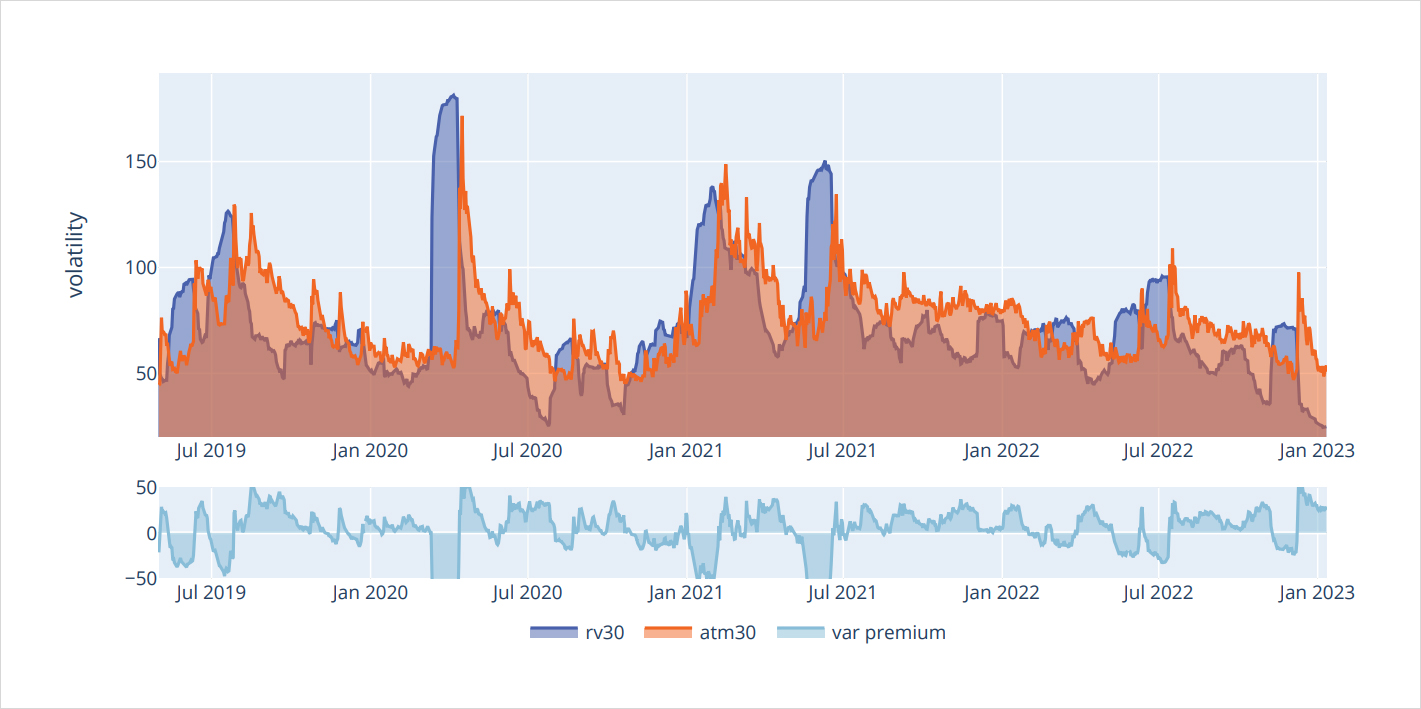
Are BTC options fairly priced in general?
In general, does implied volatility overestimate the future realized volatility?
Here we look at the VRP (variance risk-premium) in order to assess this statement.
We start by analyzing 30-day implied volatility versus 30-day realized volatility, and by shifting back IV 30- days, since IV prices future realized volatility.
Further, we break out this analysis into two buckets:
1) When the term structure is in Contango.
2) When the term structure is in Backwardation.
VRP 30 days termstructure box plot (atm shifted)
When the term structure is in Contango, the VRP has a mean of about +15pts. Meaning that 30-day ATM options are overpricing RV by +15 points (estimated $ value = 15 * Vega).
VRP 30 days skew box plot (atm shifted)
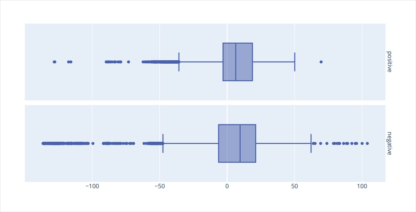
Furthermore, we analyze the VRP environment by different RR-Skew regimes. The negative RR-Skew regime has a lot more VRP noise than the positive RR-Skew regime, meaning that selling options in a positive RR-Skew environment is more certain.
VRP 30 days + skew termstructure box plot (atm shifted)
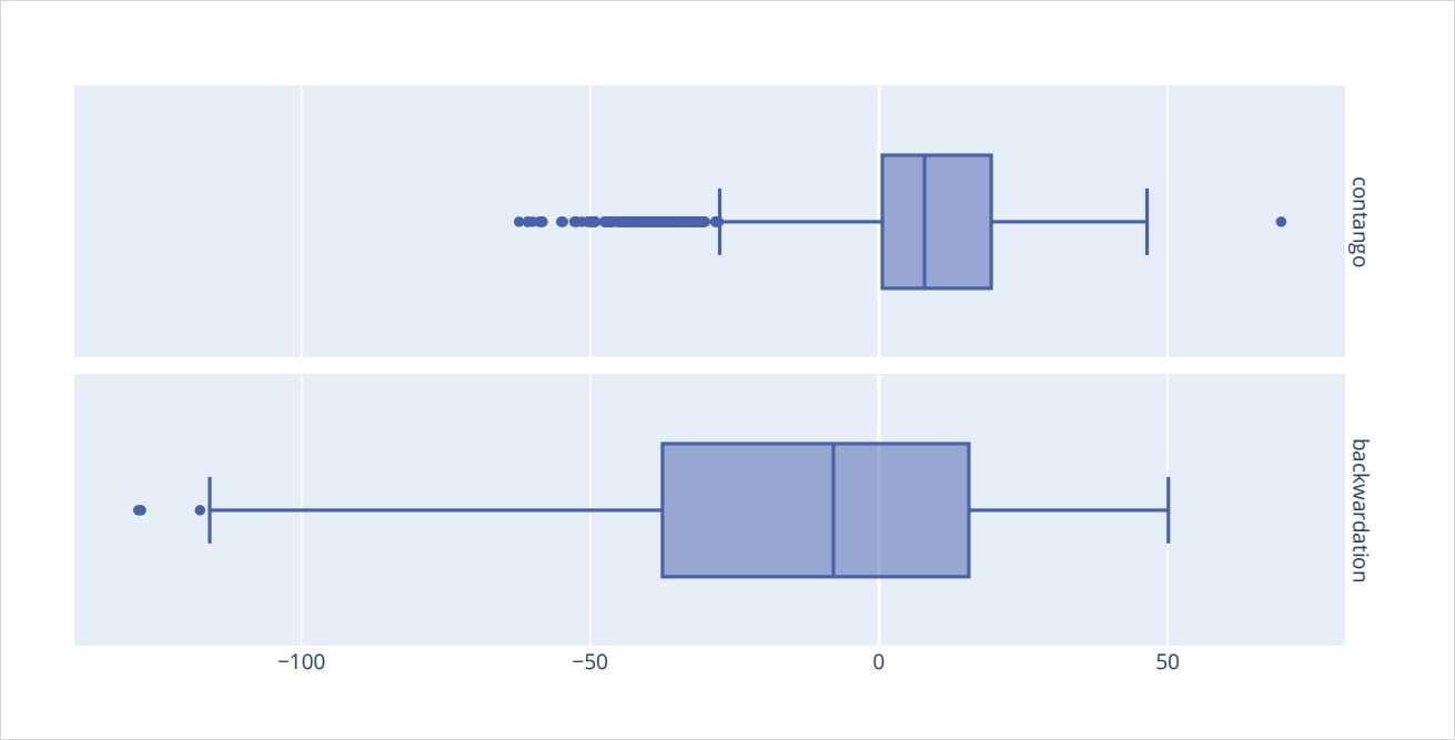
VRP 30 days – skew termstructre box plot (atm shifted)
Isolating the positive RR-Skew environment and layering the term structure regime will help us find the truly juicy VRP. We can see that there’s a slight tradeoff between Contango/Backwardation.
Backwardation in a positive RR-Skew environment has a negative VRP mean but a large potential distribution range, meaning options purchases generally are valued when spot prices explode higher with FOMO, but it’s a noisy trade.
The Contango regime provides a positive VRP but the variance of the trade truly depends on the RR-Skew regime.
Futures Basis
Deribit BTC options are actually BTC future options.
This distinction brings an additional complexity when trading BTC options, in the form of futures basis (aka the implicit interest rate).
Futures prices can move even further than spot prices as the basis expands/contracts, essentially extending delta movements a bit further.
CONSTANT BASIS annualized box plot
We can see a few interesting trends when analyzing the futures basis percentile distributions by bucketed years.
First, the basis is nearly always positive, except for outlier readings.
Secondly, we can see that 2022 was an outlier in terms of the basis “compression”.
Another peculiar insight is that RR-Skew was most volatile in 2021 and quiet during 2020. This relationship doesn’t hold for futures basis ranges, where 2020 was the most volatile and 2022 clearly compressed.
Volume and Open Interest
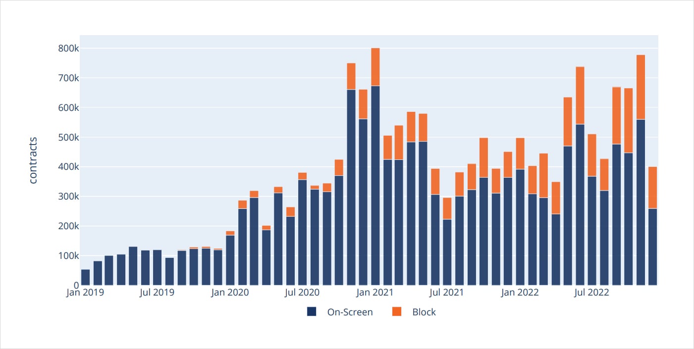
Deribit BTC monthly volumes
Deribit ETH monthly volumes
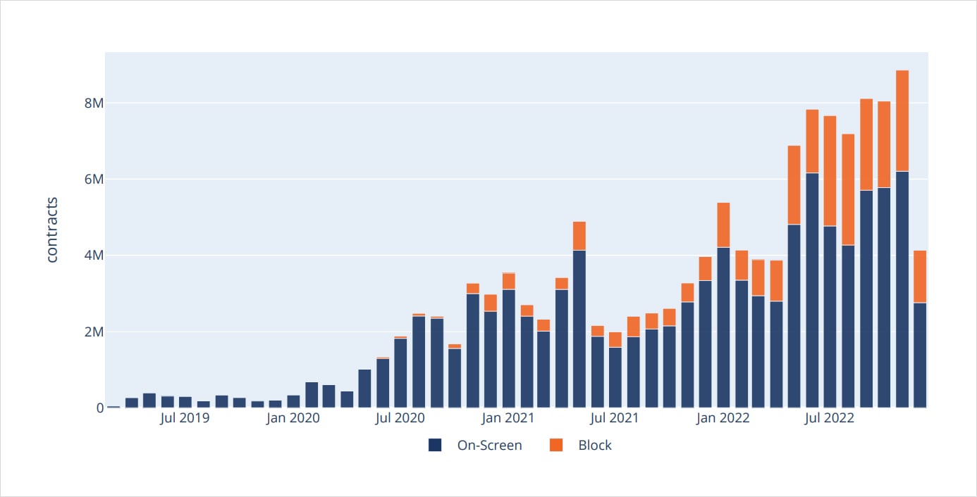
Looking at contract volumes for both BTC and ETH, we can see that monthly volumes have been growing significantly for ETH while BTC hasn’t grown much beyond the highs seen in Jan 2021.
Another interesting insight is the share of blocktrading growth for both BTC and ETH, although this is especially pronounced in ETH volumes.
Open interest btc vs eth notional $ with put/call ratio
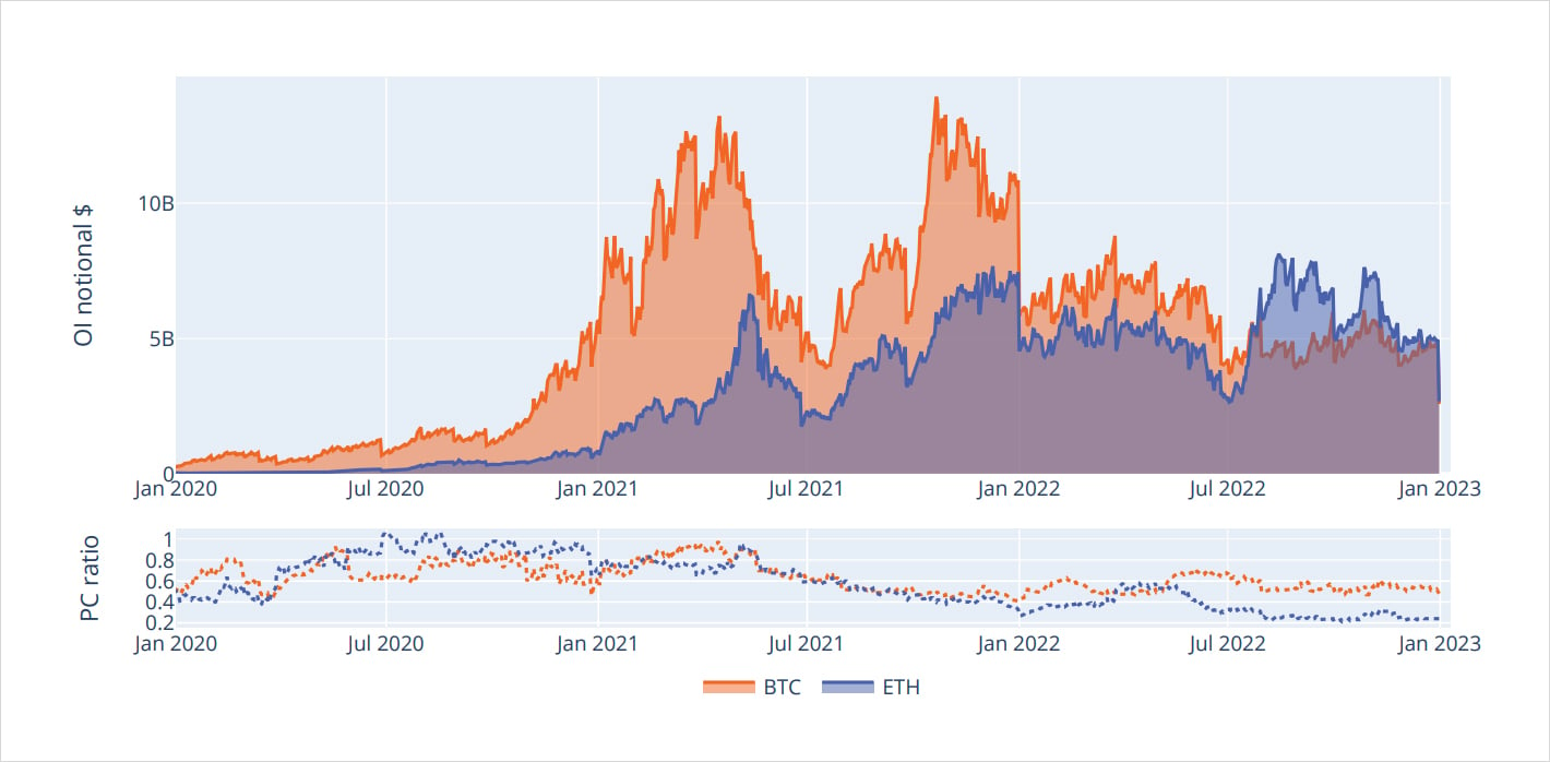
Analyzing the open interest profile, we can also see the enthusiasm for ETH options. The “flippening” occurred in July 2022 as ETH OI has outstripped BTC OI, essentially making ETH an equally important crypto volatility market.
When looking at the PC Ratio, we can see that there’s significantly more interest in ETH calls as well. This divergence is fascinating, given that the PC ratio of BTC and ETH were rather similar in the past; only around May 2022 did this divergence begin to occur and persist.
Beyond Analysis: Strategy Backtesting #1
Harvesting BTC’s Risk-Reversal Premium
By Samneet Chepal
For those in the crypto space, 2022 has not been short of surprises. Whether it be an entire L1 blockchain imploding overnight or a prominent exchange commingling user funds, the past few months have been interesting. Despite the carnage in this industry, the crypto options market is still chugging along, with traders structuring positions to speculate and hedge their risk. Unlike trading spot or futures, option structures can give traders the ability to collect income amidst choppy or bearish market conditions.
In this research piece, we will explore one of these commonly traded option structures: the risk-reversal (RR). To aid our analysis, we will reference an academic paper written by veteran option traders which outlines the profitability of trading RRs in traditional markets. For the purpose of this research, we will focus exclusively on BTC options trading on Deribit and look for opportunities to make money across both bear and bull markets. This research piece will be organized as follows:
- Overview of the Risk-Reversal Structure
- Analyze Backtested Returns
- Summary and Next Steps
Overview of the Risk-Reversal Structure
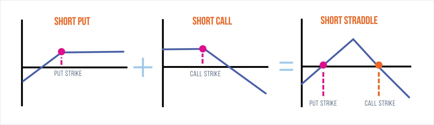
Before we delve into the details of the academic paper, it’s important to understand the mechanics of trading RRs. As shown below, we can define buying a RR as selling an OTM put and buying an OTM call (the delta of the call and put should be nearly the same).
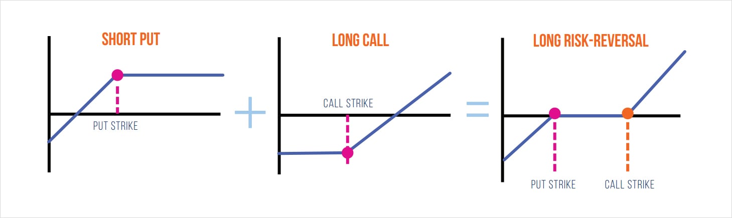
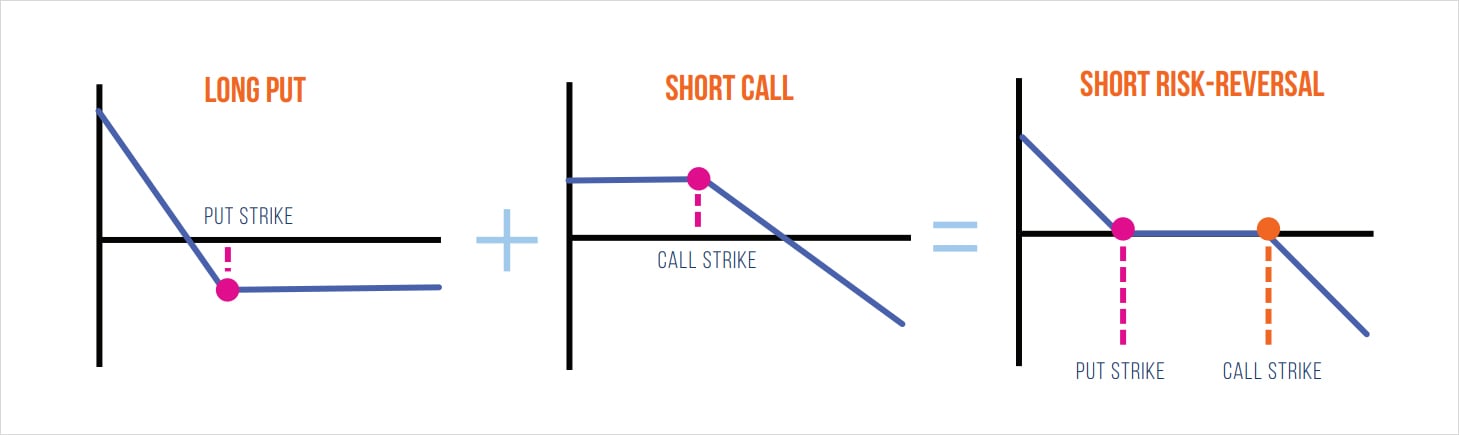
Conversely, selling a RR will involve selling an OTM call and buying an OTM put.
Depending on the strikes chosen, buying a RR is similar to being long the underlying, whereas selling the RR is similar to being short the underlying. However, as volatility traders, our primary goal is to trade volatility rather than the direction of BTC (also known as delta). For this reason, it’s common to see option traders hedge their delta exposure with futures contracts to eliminate any impact of price movements – which keeps their P&L clean and focused on trading volatility. Specifically, the hedged RR is a bet on the relative value of puts and calls.
At this point we can turn our attention to the option’s vega which will be critical in understanding the dynamics of how RRs are traded. As a refresher, an option’s vega exposure represents how much the option price will change for a 1% change in implied volatility. An option’s vega is at its peak when the option strike is near the current price of the asset. Below, we can visually analyze the net vega exposure of being long and short a RR.
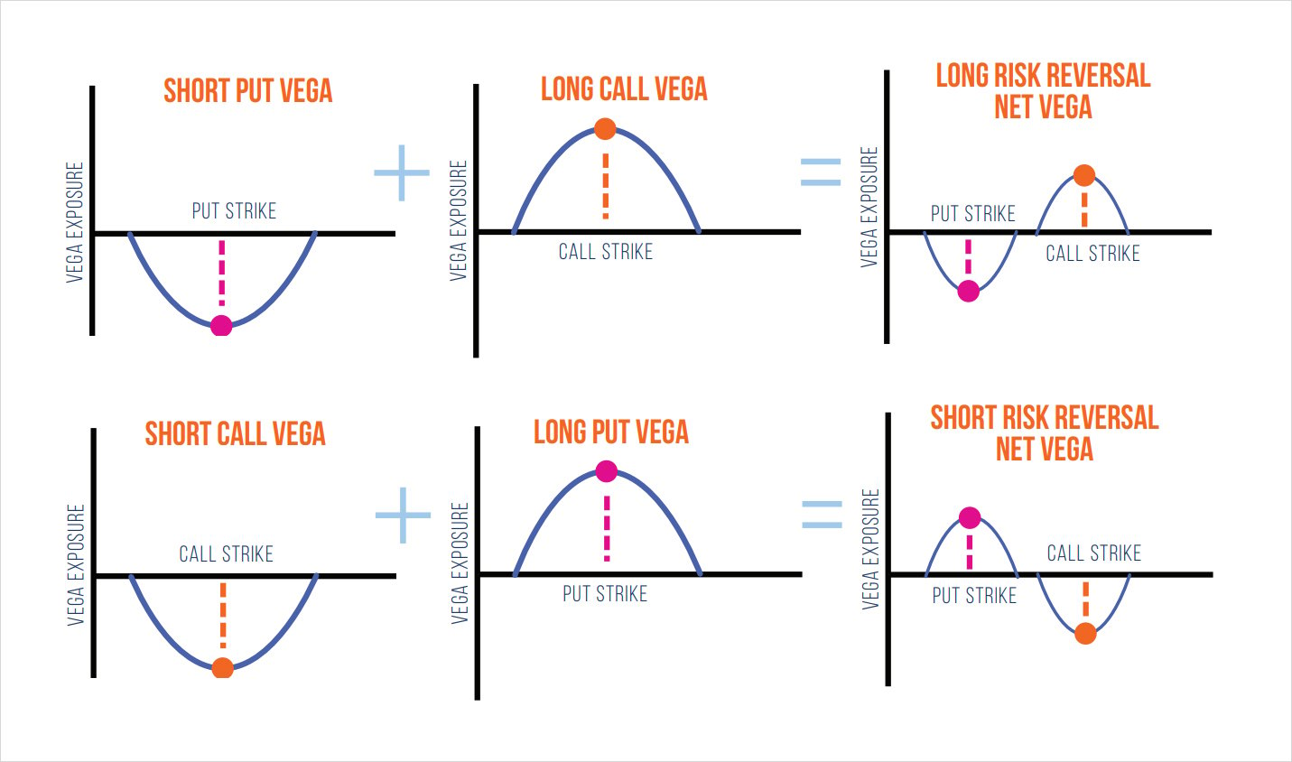
Recall that with the long RR position we are long the call and short the put. Therefore, our vega exposure to the call will reach a maximum positive value at the call strike. Conversely, given we are short the put, the vega will reach its lowest negative value at the put strike. In other words, we can say that being long the RR will benefit from positive spot-vol correlation.
Let’s consider two scenarios which encompass positive spot-vol correlation:
- An increase in BTC price is followed by an increase in volatility: as the price of BTC increases, it will approach the call strike, which will increase the vega exposure of the trade. At the same time, if implied volatility is increasing while vega is high, this will result in more profit compared to if vega was lower (ie: +vega × +vol = +P&L).
- A decrease in BTC price followed by a decrease in volatility: in a long RR position we’re short the put option; therefore, for any downside price action the net vega exposure is negative. Consequently, a decrease in volatility coupled with negative vega would result in profit (ie: -vega × -vol = +P&L).
Conversely, we can also look at this perspective from a short RR position which benefits from negative spot-vol correlation:
- A decrease in BTC price followed by an increase in volatility: in a short RR trade, as the price of BTC falls, the net vega of the long put position will increase. Therefore, it is favorable for volatility to increase as prices fall, given the trade’s positive vega exposure. (ie: +vega × +vol = +P&L).
- An increase in BTC price followed by a decrease in volatility: this would benefit the short call position because as price increases the net vega exposure to the call is reduced. At the same time, if volatility is decreasing then a net negative vega exposure will benefit from this (ie: -vega × -vol = +P&L).
Note: while this framework does not perfectly describe the spot/vol relationship in all scenarios, it can help us identify regimes where trading certain RR structures can be more favorable.
At this point, we can now discuss some of the details of the academic paper used as the foundation for this research note. The aim of “The Risk-Reversal Premium” is to demonstrate how investors can monetize the supply/demand imbalances in traditional option markets by trading RRs. Furthermore, the authors share backtested returns of each strategy and showcase how including RRs in a broader portfolio can improve the overall risk-adjusted return. The authors suggest that the risk-averse nature of investors and constant demand for downside protection causes put options to be overpriced relative to calls. To prove this hypothesis, several backtests were performed to showcase that buying the RR on index ETF options (buy the call and sell the put) outperformed the index with strong risk-adjusted returns. For this reason, the return generated by this strategy is referred to as the risk-reversal premium. Using the original paper as a foundation, we can extend this research to BTC crypto options and investigate whether these findings remain consistent.
Analyze Backtested Returns
Below are some key factors to keep in mind when interpreting the backtest results:
- The Deribit BTC options data used for this backtest ranges from 2019-04 to 2022-12. Given that Deribit BTC options are coin-denominated, all P&L will be denominated in BTC.
- The mark option price will be used to calculate P&L. This is not entirely realistic in practice; however, the objective here is to showcase whether any phenomena or inefficiencies first exist. With this knowledge, the trader can then decide on how to position accordingly.
- The target maturity for all options will be 30 days – this maturity was chosen discretionarily but generally has one of the better liquidity profiles on Deribit.
- The model will enter into the trade at the beginning of the week and select strikes closest to the user’s specified delta target. The model will then close this position after one week and roll into new strikes closer to the target delta threshold.
- Throughout the trade, the risk-reversal will be deltahedged daily based on the end of day net exposure. This is the naive baseline approach, as in practice, traders will use dynamic thresholds to execute their hedges accordingly.
From here, we can begin to analyze the first two approaches:
- Long Risk Reversal: systematically sell puts and buy calls
- Short Risk Reversal: systematically buy puts and sell calls
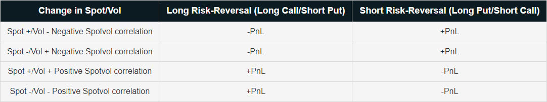
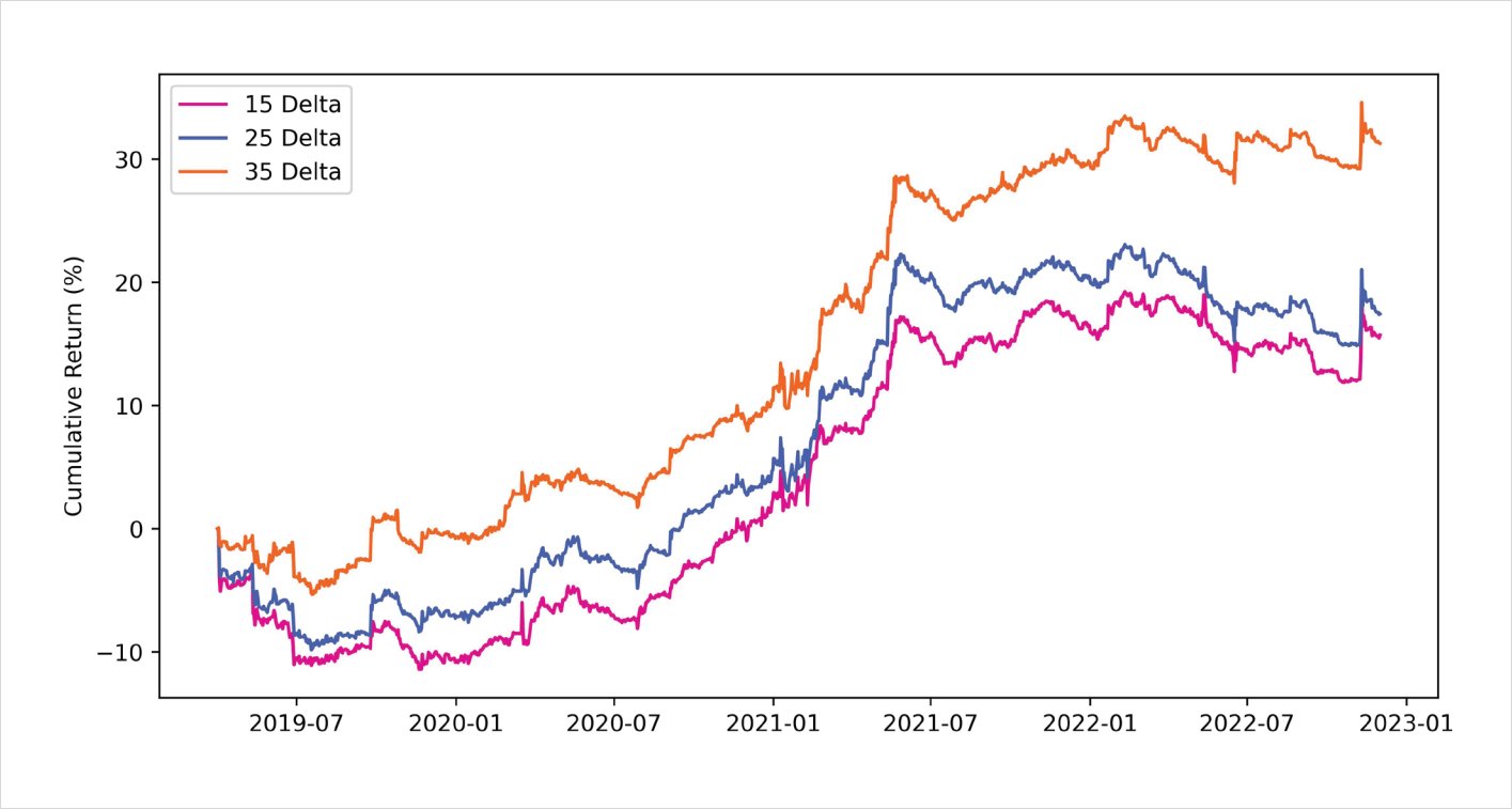
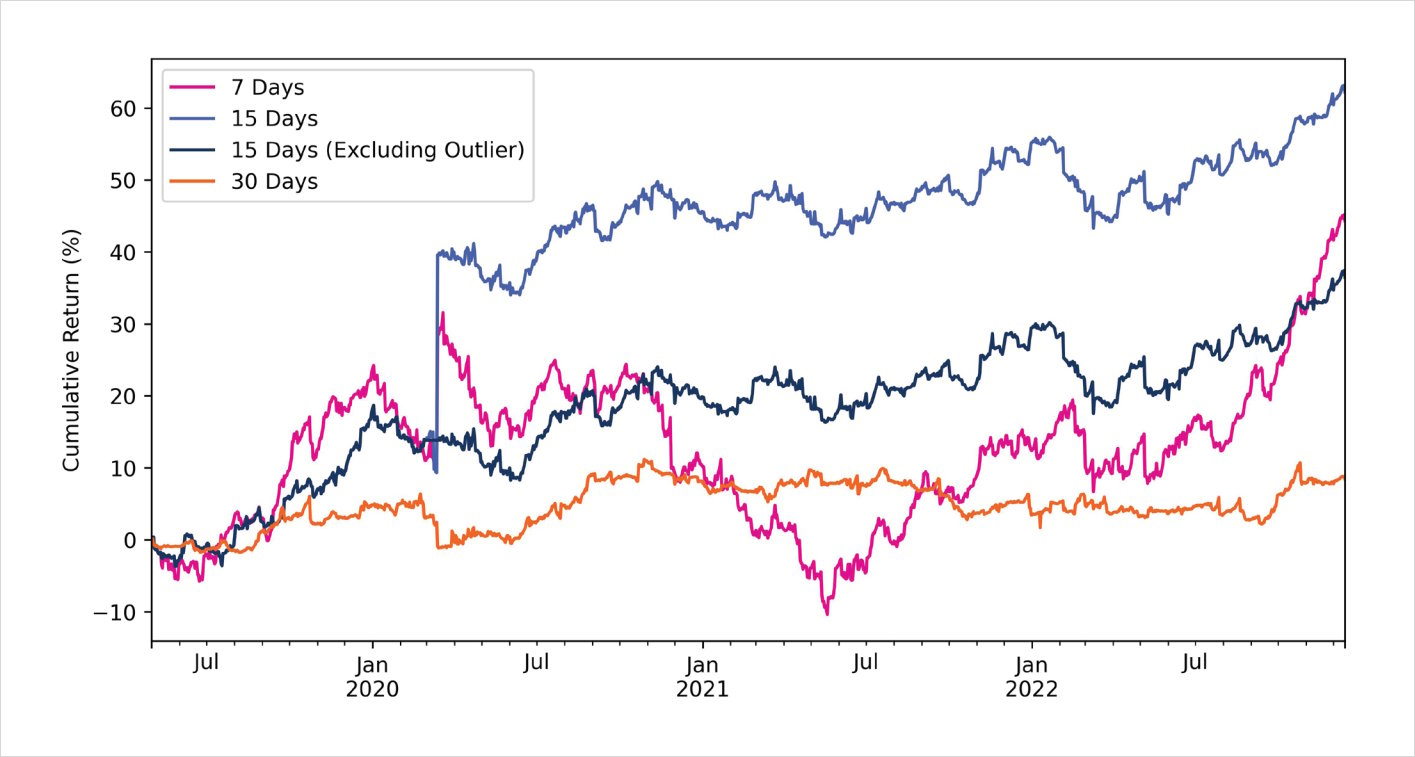
Short puts <> long calls | 30 day maturity | 2019-04-01 to 2022-12-04
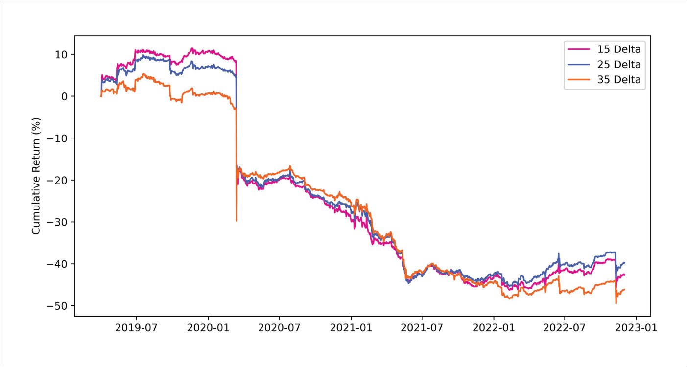
Short calls <> long puts | 30 day maturity | 2019-04-01 to 2022-12-01
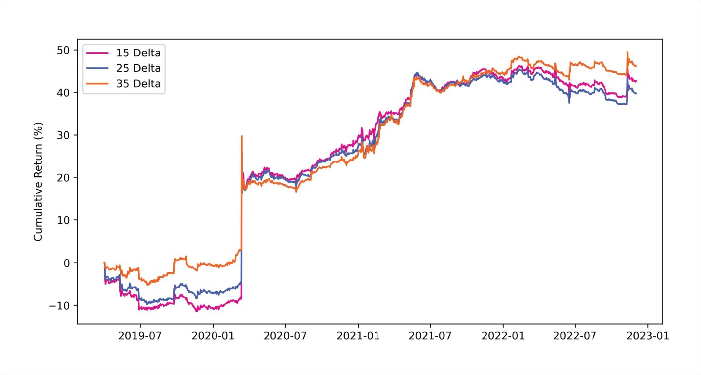
As can be seen, it’s evident that selling the RR is the better of the two approaches. The main driver of P&L stems from the model’s positioning around Black Thursday during March 2020, when the price of BTC nearly halved overnight. Even though the RR trade was hedged, the put option exploded in value and outweighed the P&L from the delta-hedge. Being short the RR would have positioned a trader very well to capitalize from this black-swan event; however, to keep things more fair, we can remove the impact of this single trade and look at the rest of the P&L. It’s interesting to note that despite removing this outlier trade, being short the RR still produces relatively strong returns relative to buying the RR.
Ex-Black Thursday:
Short puts <> long calls | 30 day maturity | 2019-04-01 to 2022-12-01
Short calls <> long puts | 30 day maturity | 2019-04-01 to 2022-12-01
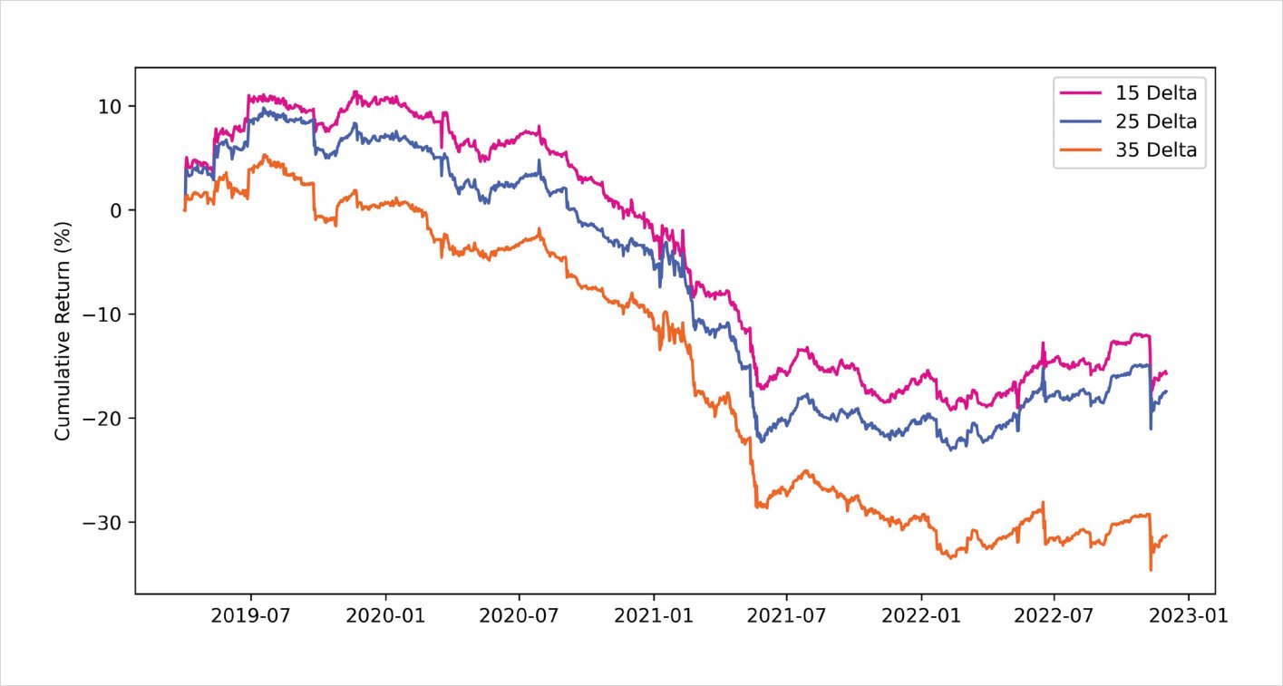
As we discussed earlier above, the performance of the RR will depend heavily on the spot-vol regime of the market. For illustration purposes, below we can see the 60 day rolling correlation between the change in daily BTC closing price and change in 1 month BTC ATM implied volatility over the past 3 years.
Rolling 60 day correlation: BTC close % change <> 1 month
BTC ATM IV % change
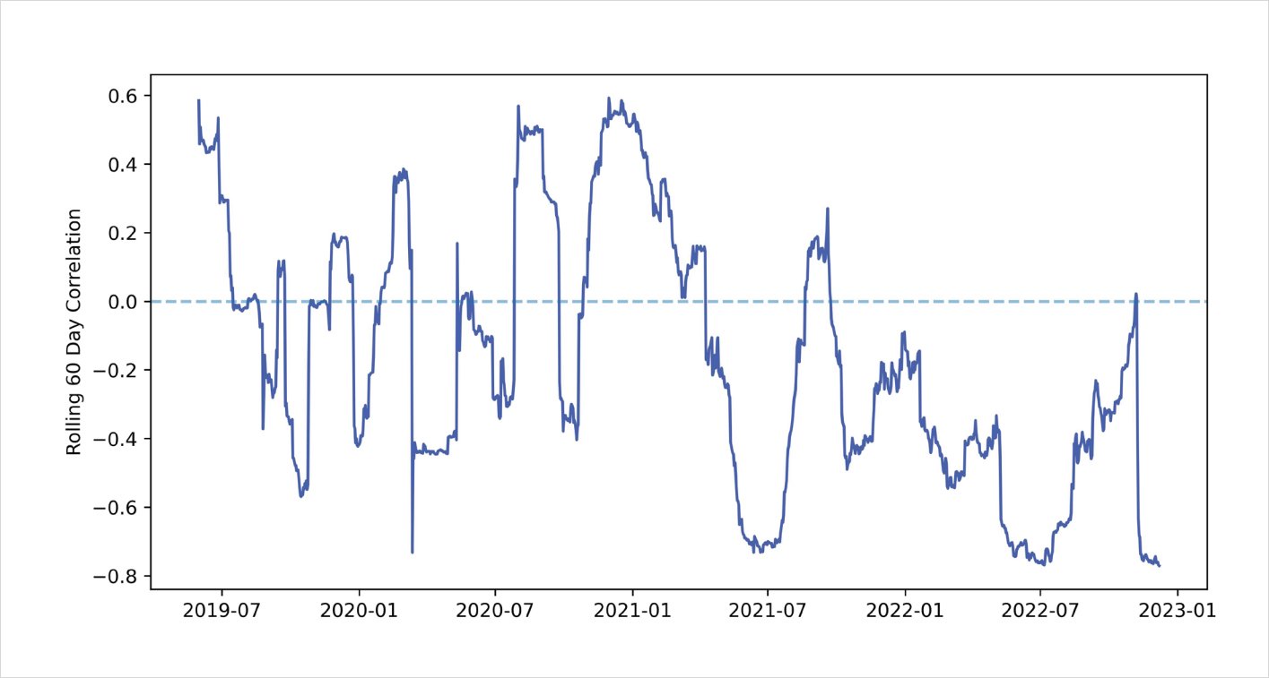
Overall, the correlation between changes in spot and changes in vol is negative 65% of the time, which makes sense when we look at the performance of the short RR trading strategy. Recall that a short RR position performs well during periods of negative spot-vol correlation. Therefore, the backtest results from above align well with these empirical findings.
At this point, we can build upon the previous two backtests and include a timing indicator, which can help filter for higher quality trades. This approach would involve using a market indicator to determine whether to buy or sell the risk-reversal. In this case, our indicator will be the z-score of the 1 month BTC skew time-series.
- The skew data is defined as: 1 month call IV – 1 month put IV (the delta of the skew will depend on the user-specified delta target – ie: for 15 delta we will use 15 delta skew)
- The z-score is calculated as: (current observation – rolling 30 day average) / (rolling 30 day standard deviation)
- Each position will be held-on for a maximum of 30 days, after which any open position will be closed to prevent stale positions
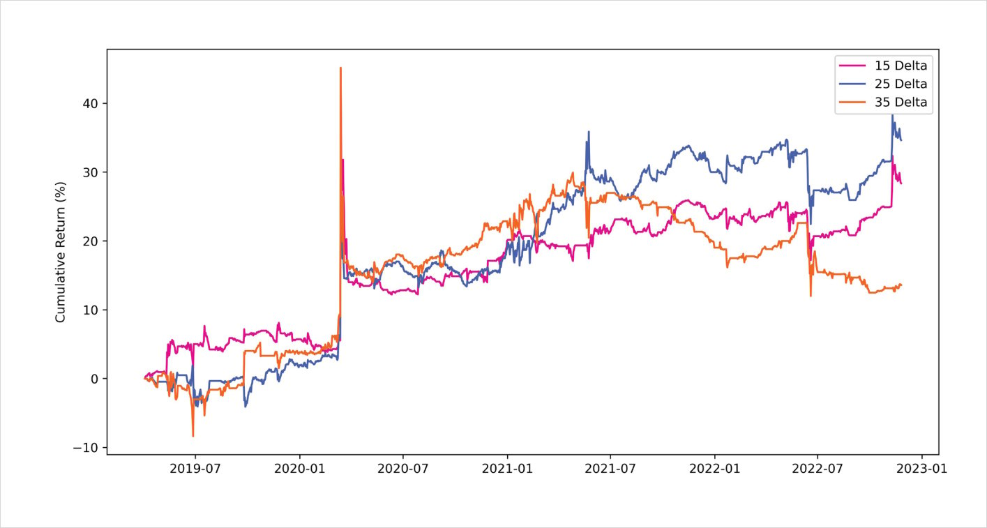
This process above helps normalize the skew timeseries into a format which can be used to identify when skew is out of line, relative to historical data points. When trading a 25 delta RR if the skew is excessively positive this implies 25 delta calls are bid higher than 25 delta puts; therefore, the model would sell the risk-reversal (sell rich calls and buy cheap puts). Conversely, when the skew is negative, then the 25 delta puts have a higher implied volatility than their respective 25 delta calls. Therefore, the model would buy the risk-reversal (sell rich puts and buy cheap calls). Below we can see the backtested returns of running this strategy with a z-score threshold of 1.00.
Risk Reversal backtest using skew entry indicator
30 days maturity | z-score = 1.00 | 2019-04-01 to 2022-12-01
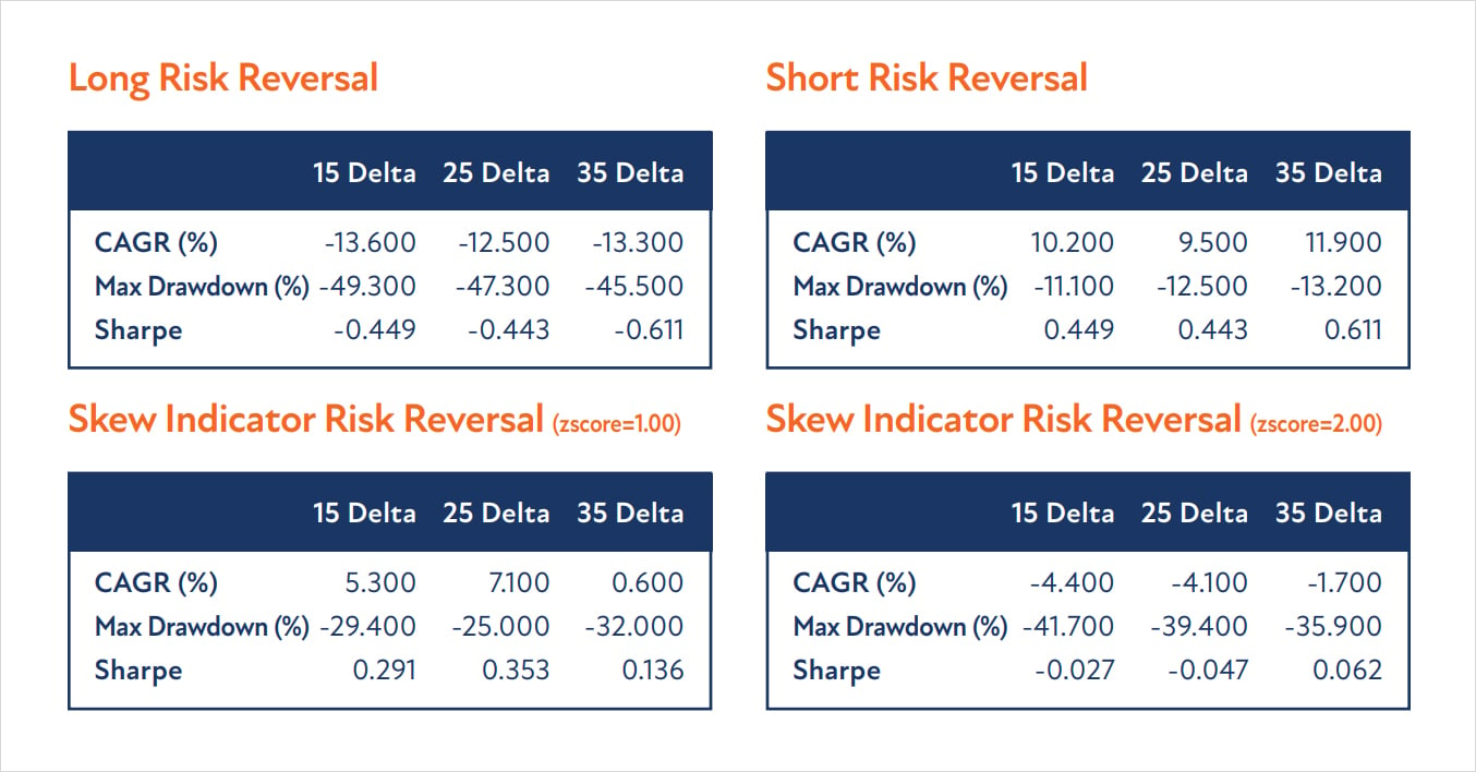
Furthermore, on a comparative basis, we can analyze the performance of the metrics across all strategies. Among the different combinations of strategies, simply selling the risk-reversal offers the best risk-adjusted returns. It should be noted that the statistics with simply selling the risk-reversal appear stable across different deltas, which may suggest more robustness compared to the skew indicator model.
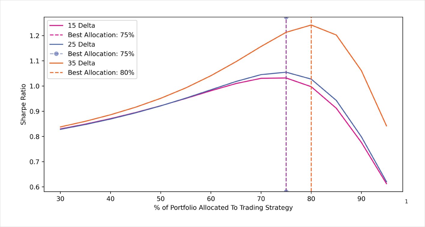
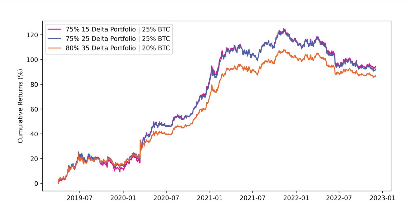
One final study that we can perform is analyzing the performance of combining the RR strategy with a long BTC position. Given that selling the RR had consistent returns across all delta thresholds, we will use this strategy for our portfolio analysis.
The goal here is to determine the optimal weighting for the trading strategy in the overall portfolio. Below is a diagram outlining the optimal allocation to the RR trading strategy. In the cases below, an allocation anywhere between 75% to 80% dedicated to the trading strategy and the remainder to spot BTC offered the best risk-adjusted returns using the Sharpe ratio.
Optimal portfolio allocation: BTC + Short call and long put
Optimal risk-adjusted portfolio cumulative returns: BTC + short call & Long put
Conclusion and Next Steps
Overall, it’s interesting that unlike traditional markets, systematically selling risk-reversals across time offer strong risk-adjusted returns. This can likely be explained by BTC’s strong call skew during the early 2021 bull-market, in addition to several market shocks which greatly rewarded buyers of puts. However, as the crypto options market matures with new institutional participants, it’s reasonable to expect a different regime for trading risk-reversals given the change in supply/demand dynamics. As a result, these strategies will likely become less profitable and new approaches will be required to squeeze out marginal alpha.
Acknowledgments
Greg Magadini, Euan Sinclair, and Ben Moussa for their insightful comments and suggestions on this research piece.
Beyond Analysis: Strategy Backtesting #2
Systematic Volatility Trading With BTC Options
By Samneet Chepal
One of the benefits of systematic trading is that it provides investors with a clear plan on how to execute their trading strategy. Having a good understanding of a strategy’s historical performance and expected future returns across various market conditions can provide greater ease to a trader, especially during abnormal volatility. In this research piece, we will analyze the backtested performance of several systematic volatility trading strategies tailored to the BTC options market. While all of these approaches will be purely systematic, discretionary traders can take note and use these insights to further refine their trading approach.
This piece will be structured as follows:
- Systematically Selling Straddles
- Systematically Selling Butterfly Spreads
- Event-Driven Long-Volatility Bets
- Overview and Conclusion
Systematic Straddle Trading
A straddle is a popular options structure which allows traders to make bets on the future volatility of the underlying asset. A trader buying the straddle will purchase a call and put option closest to the current price of the underlying, with the expectation of realized volatility being higher, relative to the current implied volatility. It’s a well-known observation that the market anticipates future volatility to be higher than actual volatility. In other words, the volatility implied by the options market is typically higher than the actual realized volatility over the long-run. As shown below, since April 2019, the implied volatility for 30-day BTC options has been greater than 30-day realized volatility for nearly 70% of the time. Given this behavior, it would make more sense for us to sell straddles to profit from the market’s tendency to overprice implied volatility.
BTC IV/RV 30 day maturity vol spread: 2019-04-01 to 2022-12-07
The results below showcase the backtested performance of selling straddles across different maturities. Given that this strategy aims to be delta-neutral, the model will hedge only after the index price moves past a certain threshold. This is common industry practice as it allows the delta of the position to fluctuate, and thereby reduces transaction costs associated with constant hedging (in this case, we’ll set our threshold to hedging the delta after every 2.5% change in BTC price).
Systematic BTC straddle selling (2.50% hedge threshold)
2019-05-01 to 2022-12-04
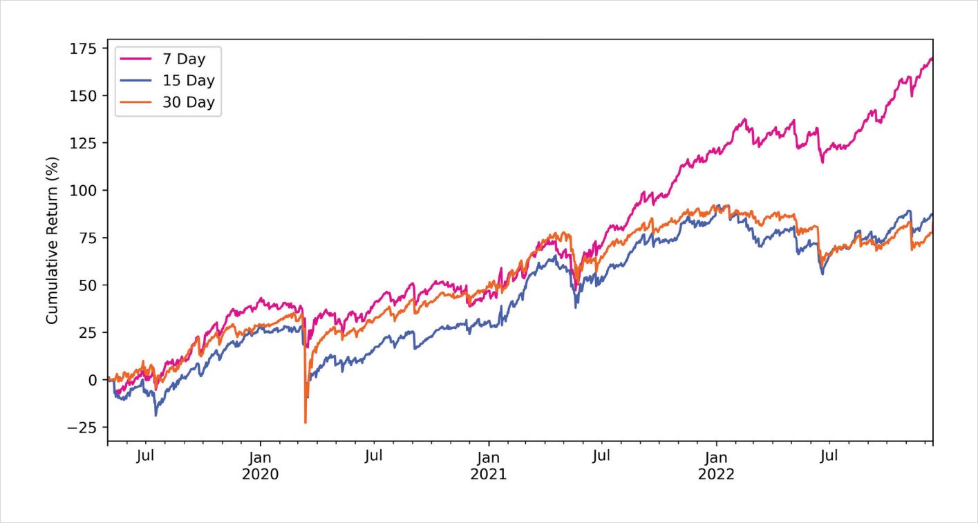
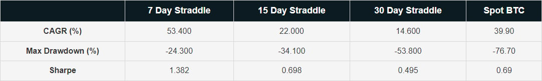
Despite several crashes over the past years, this strategy performs well over the backtested period with strong risk-adjusted performance. Empirically, this makes sense, as selling options allows traders to collect premium and compound gains over time. As can be seen below, the performance of the weekly straddle strategy offers good risk-adjusted returns compared to simply holding BTC.
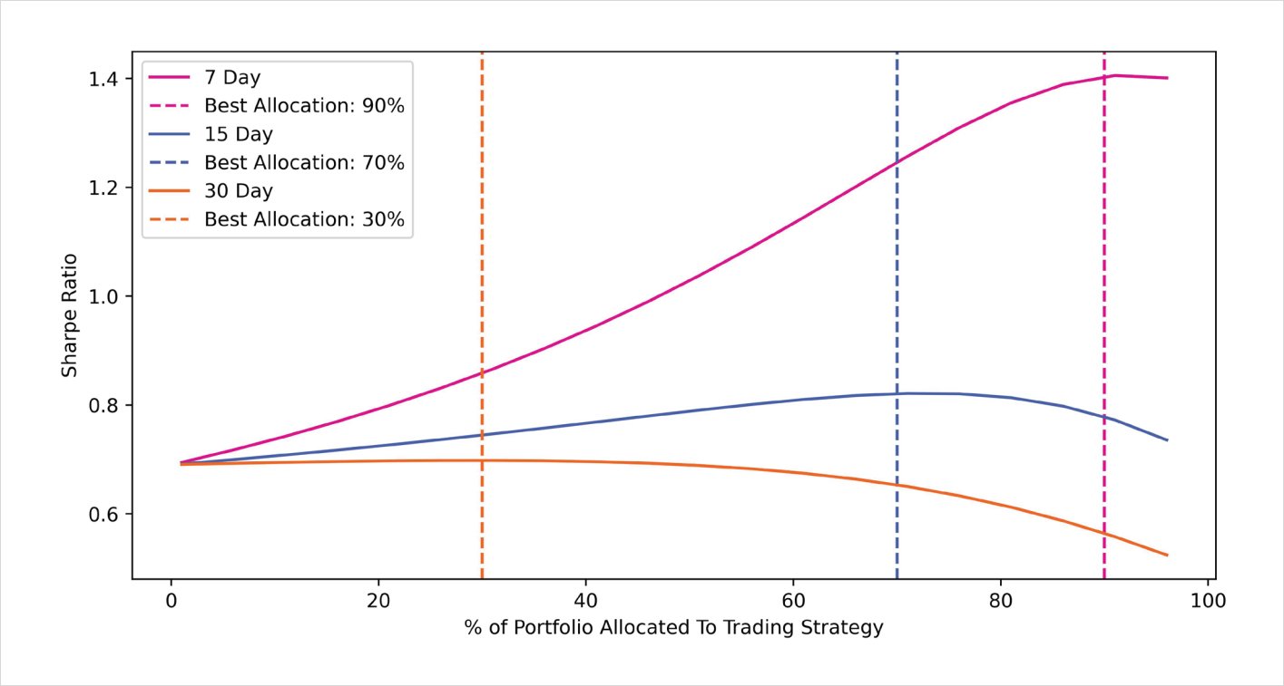
It should be noted that naively selling volatility like this has led to disastrous outcomes when the risk is not properly managed. Selling straddles can in theory lead to unlimited losses, given that volatility can skyrocket to levels which were previously not observed. The primary reason for the blow-up of these vol-selling strategies revolves around their excessive use of leverage. For example, selling straddles with the goal of collecting “stable income” can work in many cases; however, extreme market volatility (which occurs more often than implied by the options market) can completely erode all profits. As a result, it would be advisable to allocate only a fraction of the portfolio to volatility selling. Below, we can observe the optimal weight for the straddle selling strategy in a broader portfolio of spot BTC.
The maturity selected has a significant impact on how much we should allocate to the portfolio for optimal risk-adjusted returns. In this case, the weekly straddle selling strategy comprises nearly 90% of the portfolio paired with 10% spot BTC. Conversely, for longer-dated monthly straddles, the strategy only needs to have a 30% allocation before the Sharpe ratio begins to decline. Approaching volatility harvesting with this framework is likely more sustainable and can help investors tolerate future drawdowns with greater ease.
Optimal portfolio allocation BTC + Short straddle
Systematic Butterfly Trading
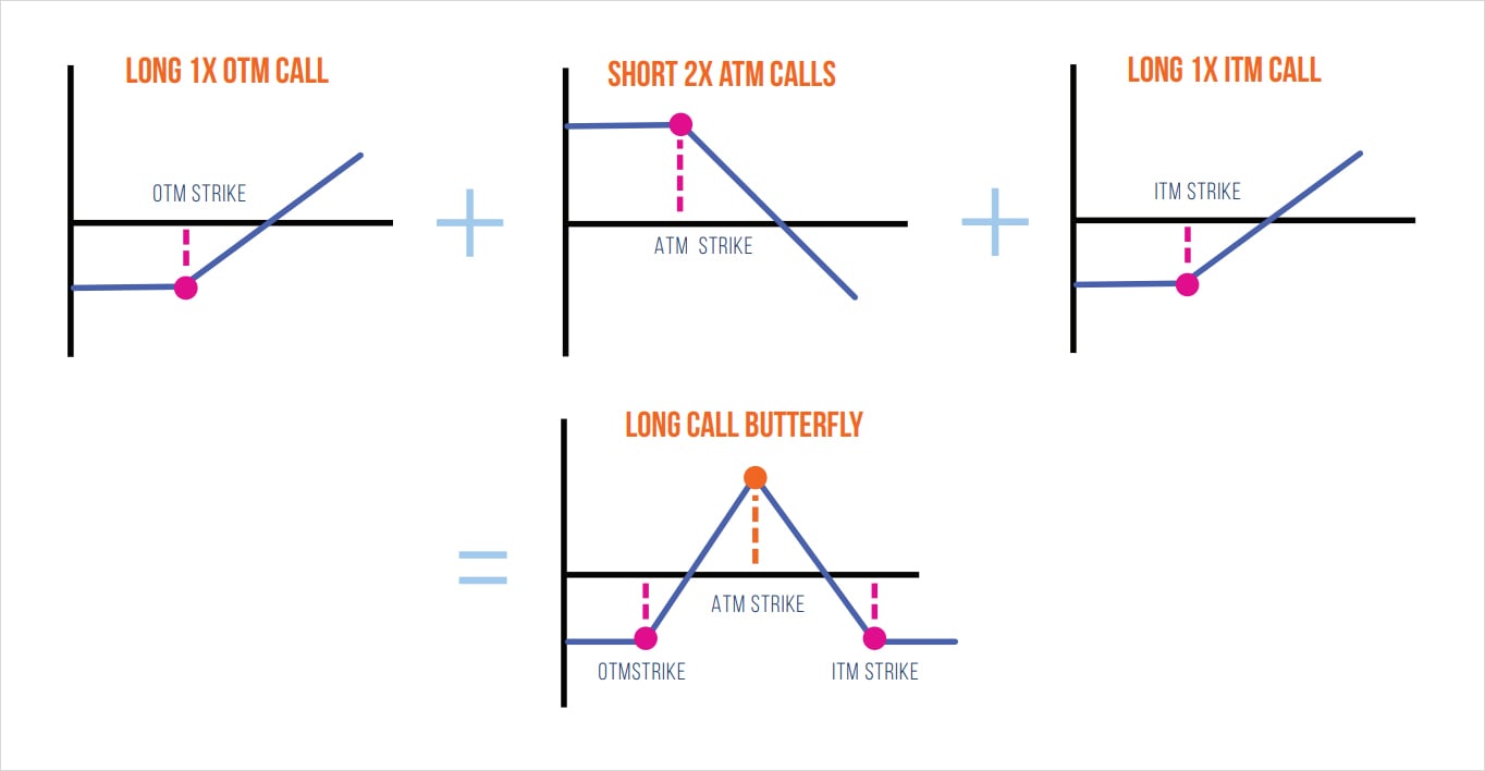
Although selling straddles can earn decent returns over a long enough time period, the amount of risk inherent with this strategy may not be tolerable to specific investors. In this case, butterfly structures can offer a similar payout structure to the straddle, except that the infinite downside risk is capped at the expense of lower profits. This structure involves selling two calls near the current price of BTC and buying a call slightly below and slightly above the current price (ideally they are equidistant to make the payoff equal). For the purpose of our backtest, the OTM and ITM strikes will be 10% away from the current price of BTC. Note: this butterfly structure can also be replicated using put options.
Following the same delta-hedging logic as the straddles above, we can see that the P&L associated with this approach offers decent returns over the backtest period, however, the results across different maturities have significant variance. After adjusting for a key outlier trade, we can see that even the best performing strategy fails to beat the performance of the worst performing straddle strategy. The lower overall returns relative to the straddle strategy makes intuitive sense because, in this case, we have to buy two options which significantly erodes P&L due to theta decay. Although downside risk is limited with this approach, investors are likely better off selling straddles but adjusting their position size accordingly to a point where the portfolio risk is in line with their desired thresholds.
BTC Butterfly +/- 10% strikes | 2.50% hedge threshold
2019-05-01 to 2022-12-14
Event Driven Volatility Trading
As discussed above, it is usually more profitable to be short options given that implied volatility tends to be higher than realized volatility. However, there are unique situations where being long volatility before key events can lead to profitable trading opportunities. In this case, we’ll explore the P&L of systematically buying volatility a week before key economic data releases such as CPI and Fed decisions.
To execute this strategy, we will buy an ATM call option one week before a key economic event. The option will be hedged based on a 2.50% threshold approach, as discussed in the straddle strategy. The logic here is that in the days leading up to the event, the market may have uncertainty on the outcome – leading to greater realized volatility in the underlying. We would want to close this position a day before the actual event to avoid the postevent volatility sell-off. In both crypto and traditional option markets, it’s common to see a “vol crush” after key economic events have passed, as the market now has less uncertainty to digest.
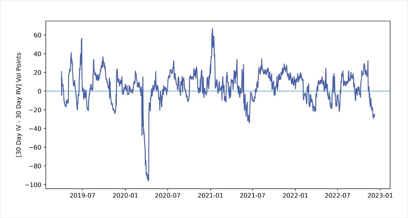
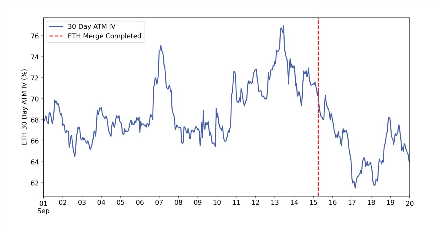
For example, recall earlier in the summer of 2022 when ETH was moving to Proof-of-Stake. In the days leading up to the event, the options market was pricing higher volatility, given the uncertainty associated with whether the Merge was actually going to happen. Shortly after the event, ETH IV plummeted once the market was convinced the Merge went through successfully.
ETH 30 day constant maturity ATM IV: 2022-09-01 to 2022-09-30
Ever since the FOMC started raising interest rates back in November 2021, crypto markets have been highly reactive to key economic releases (ironically, for an asset class that prides itself in decentralization, trading crypto over the past year has been highly dependant on the outcome of a single institution – the Fed!). Below we can see the performance of this strategy individually on CPI and FOMC events.
Buying volatility 7 days before FOMC release date 2021-11-01 to 2022-12-13
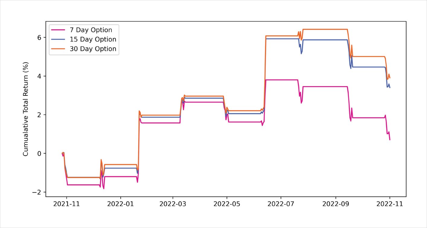
Buying volatility 7 days before CPI release date 2021-11-01 to 2022-12-13
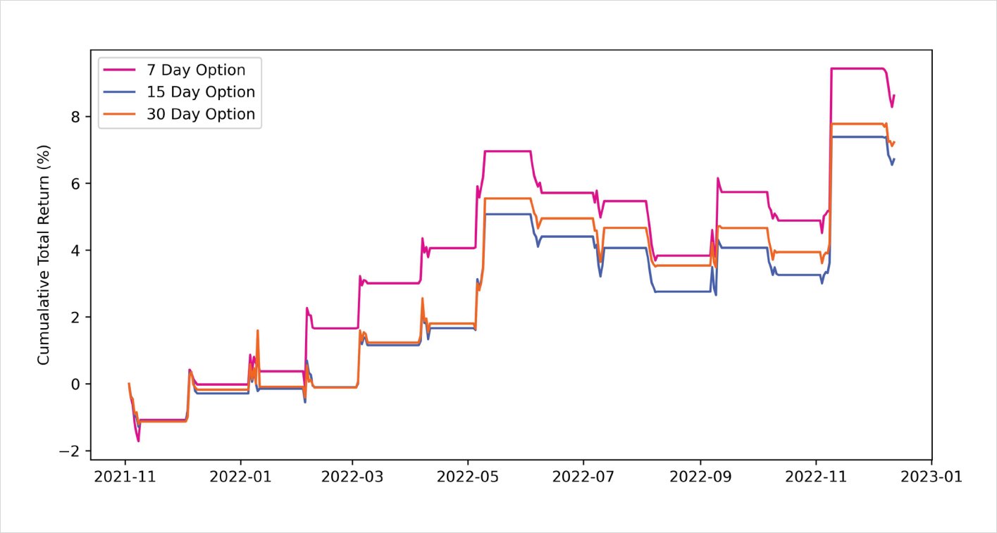
While the performance of this trading strategy is nowhere close to the straddle selling approach, it should be noted that there have been less than 15 trades for each individual backtest. Therefore, the small sample size makes it too early to conclude whether this strategy will continue to work in practice – we need more data to reach statistical confidence on the effectiveness of this strategy. However, observing the overall positive returns across both approaches may suggest there is some benefit to being positioned in a long-volatility structure before key macro events. If anything, these long-volatility bets may enhance or serve as a hedge against existing short-volatility strategies in a broader portfolio.
Conclusion
Despite running different backtests and scenario analysis, ultimately, a strategy’s success comes down to whether an investor decides to proceed forward. Although these strategies above are oriented towards systematic investors, discretionary traders can also find benefit in using a quantitative approach towards framing their investment framework. For example, while a discretionary trader may have strong intuition on the nature of a particular market, having a baseline figure for the risks and returns of a given strategy can provide further validation of a strategy’s effectiveness and give the trader more confidence to increase their position size accordingly. Overall, as the derivatives market in this space continues to grow with new underlyings, greater liquidity, and new products (ie: exotic options, variance swaps etc…), we can expect further opportunities to quantify new systematic strategies which investors can add to their crypto portfolios.
Disclaimer
This report provides data and analysis to the user to facilitate the user’s own investment decisions. It does not attempt to provide investment advice or recommendations. Any interpretation of the data presented that leads to an investment is at the user’s own risk and Amberdata can not be held responsible for any losses that occur from such investments.
Important notice! Crypto currencies and options markets have large potential rewards, but also large potential risks. You must be aware of the risks and be willing to accept them in order to invest in crypto currencies and options markets.
Don’t trade with money you can’t afford to lose. This is neither a solicitation nor an offer to buy/sell crypto currencies or options.
All information from Amberdata is obtained from sources believed to be accurate and reliable. However, errors or omissions are possible due to human and/or mechanical error. All information is provided “as is” without warranty of any kind.
Amberdata and its information partners make no representations as to accuracy, completeness, or timeliness of the information on this site.
Amberdata does not represent or endorse the accuracy or reliability of any of the information, content or advertisements (collectively, the “Materials”) contained on, distributed through, or linked, downloaded or accessed from any of the services contained on this website (the “Service”), nor the quality of any products, information or other materials displayed, purchased, or obtained by you as a result of an advertisement or any other information or offer in or in connection with the Service (the “Products”).
THANKS TO
Greg Magadini – CFA, Fabio Bassani, Tony Stewart, Euan Sinclair, and Samneet Chepal – CFA