

As you may have guessed, a short straddle is the exact opposite of a long straddle. In the previous lecture we were trading a long straddle, but the trader on the other side of that trade, i.e. the person who sold us the long straddle, was by definition entering a short straddle with the same parameters.
A short straddle is usually initiated as a price neutral strategy, and will typically have a delta close to zero when it is opened. The strategy is also bearish on volatility. Ideally when entering a short straddle, we want the underlying to move as little as possible, and implied volatility to drop. The strategy is constructed by:
-Selling a call option with strike price A
-Selling a put option with strike price A
Both options have the same expiry date, and the underlying price is typically somewhere close to the strike price A.
Both options are sold and therefore a net credit is received when we open the short straddle. This gives us a payoff chart that looks like this.
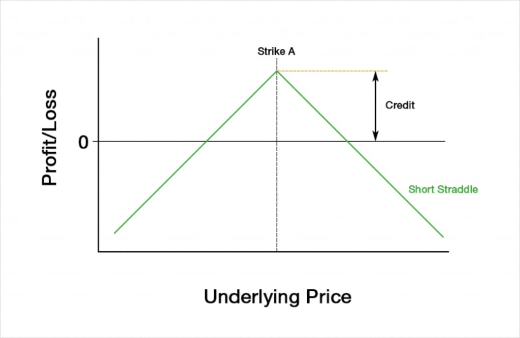
The profit is capped at the premium collected, and the maximum profit will only occur if the underlying price is precisely at the strike price at expiry.
The maximum loss is uncapped in both directions (other than by the underlying price reaching zero to the downside), and in dollar terms the payoff is symmetrical either side of the strike price. We have sold both the put and the call, meaning a much larger net credit has been paid than if we had chosen just one to sell. However, we now have risk in both directions of course.
If we hold the short straddle until expiry with no further adjustments, it is simply a bet that the underlying price will not have moved outside of a certain range. This range is determined by our two breakeven points. In dollar terms, the breakeven points can be calculated as:
First Breakeven = Strike price – Premium
Second Breakeven = Strike price + Premium
These breakeven points are exactly the same for the buyer and seller of the straddle (ignoring fees).
The Greeks
We can add our Greek values for the put at strike A to the values for the call at strike A, and this will give us the total Greek values for the short straddle.
To analyse how the Greeks of the short straddle behave we will use the same figures as we used for the long straddle in the previous lecture:
Underlying price: $100
Time to expiry: 50 days
Interest rate: 0
Implied volatility: 60%
Strike A: $100
Profit and loss
With these parameters, selling the $100 straddle will initially give us a credit of about $17.68. The payoff chart looks like this.
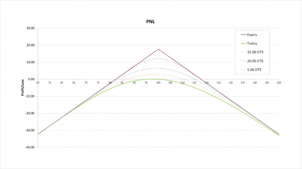
The maximum profit is capped at the premium collected, which is $17.68. The maximum profit occurs when the underlying price is precisely at the strike price of $100 at expiry.
To the downside, the maximum loss is only capped if the underlying price reaches zero, and the maximum loss is completely uncapped to the upside. The further the price moves in either direction the bigger our loss at expiry will be.
There are two breakeven prices, one to the upside and one to the downside. The one to the downside is calculated by subtracting the total premium collected from the strike price, which gives us:
$100 – $17.68 = $82.32
The breakeven price to the upside is calculated by adding the total premium collected to the strike price, which gives us:
$100 + $17.68 = $117.68
Delta
As with the long straddle in the previous lecture, the short straddle can have either a positive or negative delta. The sign of the delta depends on where the underlying price is relative to the strike price.
This chart shows the delta of the short straddle, with the x axis being the underlying price. The extra lines also show how the delta will evolve as time passes.
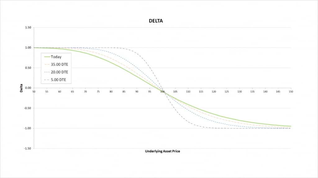
When the underlying price is close to the strike price, the positive delta gained from selling the put and the negative delta gained from selling the call largely cancel each other out. The total delta for the short straddle is therefore very small when the underlying price is close to the strike price.
When the underlying price decreases, the positive delta from selling the put option increases in magnitude, whereas the negative delta from selling the call decreases in magnitude. Both of these have the effect of making our total delta increasingly positive as the underlying price decreases. The more the underlying price decreases, the more positive our delta becomes, meaning we effectively get more long the underlying as the price decreases. Eventually the delta of the deep OTM call approaches 0, while the delta of the deep ITM put approaches -1. As we are short both, this means our total delta approaches 1 as the underlying price continues to decrease.
Conversely, when the underlying price increases, the positive delta from selling the put decreases in magnitude, whereas the negative delta from selling the call increases in magnitude. Both of these have the effect of making our total delta increasingly negative as the underlying price increases. The more the underlying price increases, the more negative our delta becomes, meaning we effectively get more short the underlying as the price increases. Eventually the delta of the deep OTM put approaches 0, while the delta of the deep ITM call approaches 1. As we are short both, this means our total delta approaches -1 as the underlying price continues to increase.
So by being short a straddle, we are effectively speculating that the market will be range bound, and will not trend. The more the market trends, the more the short straddle will lose.
As time passes the price range where delta is anything other than 1 or -1 gets narrower, and the delta delta line gets much steeper, meaning delta changes much faster within this smaller range.
Gamma
As we move from left to right on the delta chart, the delta of the short straddle is always decreasing. This means the gamma for a short straddle is always negative.
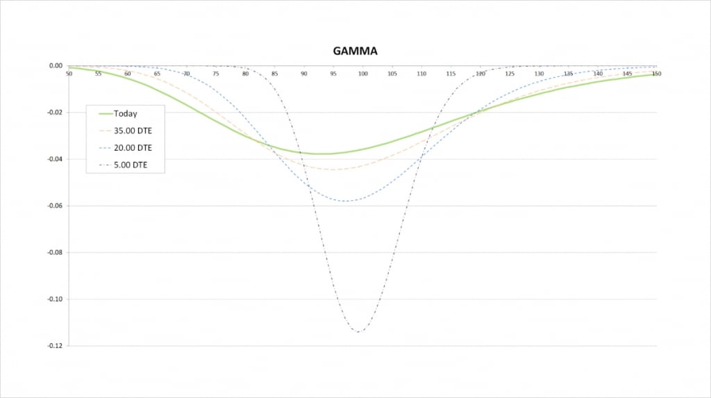
The steeper the delta line, the more extreme the gamma is. The delta line is steepest when we are relatively close to the strike price, so this is where gamma peaks in magnitude.
When we get much closer to expiry, the price range where there is any significant delta is much narrower, and delta changes much quicker. On the gamma chart this results in a narrower price range for significant gamma, and much more extreme values of gamma due to the more rapid changes in delta. The less time until the options expire, the closer the peak in gamma will be to the strike price.
Vega
We are short both a put and a call. Both of these legs have negative vega, so our total vega for the short straddle is always negative, and always of a greater magnitude than for either of the two individual options.
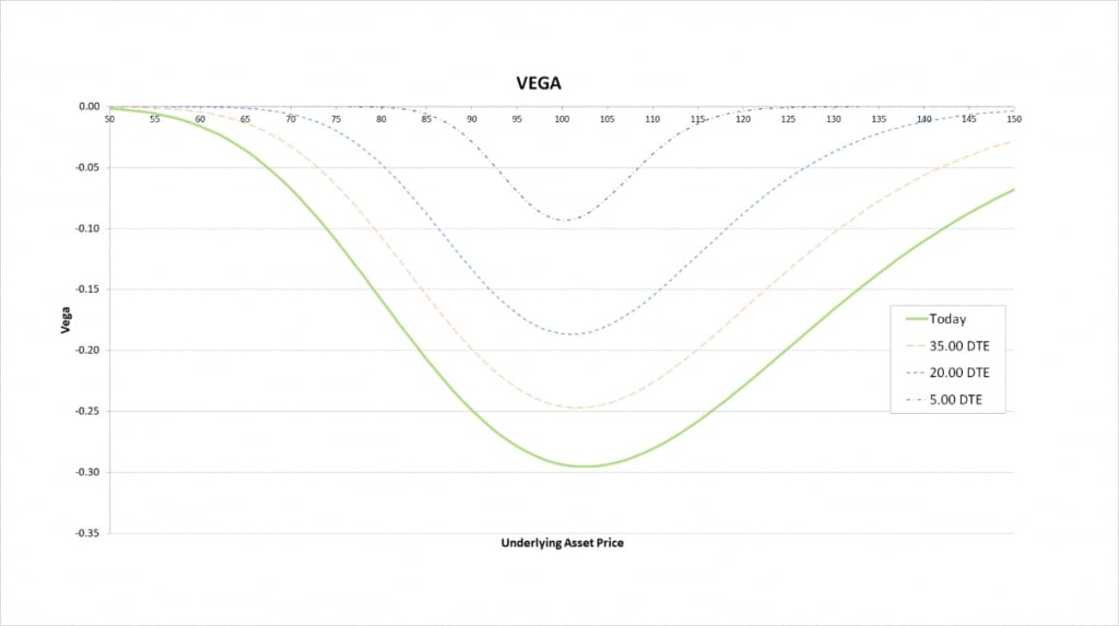
The seller of any option has a negative vega. The magnitude of this vega is greatest when the option is close to the money, and as time passes, the magnitude decreases no matter where the underlying price is in relation to the strike price.
The short straddle clearly suffers from an increase in implied volatility, and benefits from a decrease in implied volatility. If all else remains equal and implied volatility increases, both the put and the call will increase in value, resulting in a double loss for our short straddle.
Theta
Theta is the major advantage to a short straddle. All short options have positive theta, meaning they gain value as time passes. With a short straddle we are short a put and a call, resulting in two legs where we gain from theta. It’s also only possible for one of them to be ITM at expiry so at least one of them is guaranteed to lose all of its value by expiry.
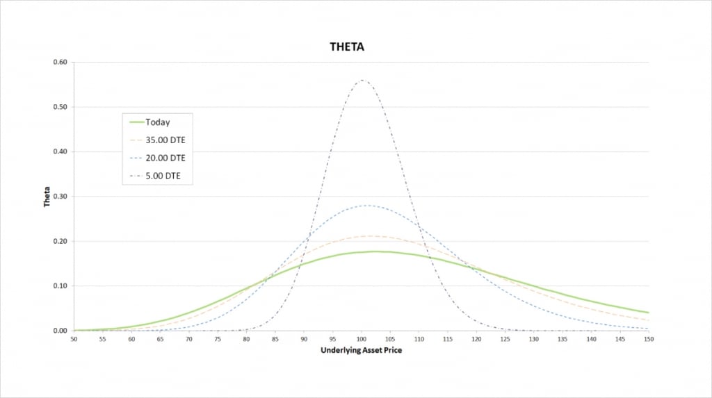
The theta is greatest when the underlying price is close to the strike price. This is where the options will have the most extrinsic value, and therefore the most value to lose to time decay. When we initially open the short straddle we will typically be using ATM options, so they are likely to have plenty of extrinsic value to lose as time passes. As the seller of both options, their loss of value represents a gain for us.
As time passes, the price range where there is any significant theta gets smaller, and the peak theta is of a greater magnitude.
As the seller of a straddle, we want the underlying price to stay range bound. When we hold the short straddle until expiry, if the underlying price has failed to move far enough away from the strike price, we make a profit. However, if the underlying price is outside of our breakeven range, we make a loss.
Inverse option contracts
A short straddle consists of a short put and a short call. The same is true when using the inverse option contracts on Deribit.
This chart shows the bitcoin payoff at expiry of a long straddle using the bitcoin options on Deribit. In this example we’ve sold one call option with a strike price of $50,000, and sold one put option also with a strike price of $50,000. We collect 0.05 BTC for each option, and therefore collect a total of 0.1 BTC for the short straddle. This is the exact opposite of the position we looked at in the previous lecture.
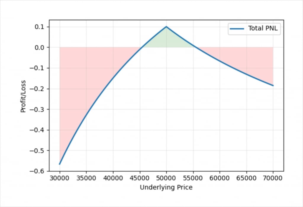
The shape of the profit/loss in bitcoin terms is similar to the profit/loss in dollar terms that we saw earlier. Due to the nature of payoffs with inverse contracts, the line is curved instead of straight, and we can also see that if the underlying price decreases, we lose far more bitcoin than for an equivalent increase in price. This is due to how much bitcoin it takes to pay a fixed amount of dollars when the underlying price is different.
For example, if the underlying price is $20,000 lower than our strike price at expiry, and is therefore at $30,000, our $50,000 put is worth $20,000. As the underlying price is now $30,000, $20,000 is the equivalent of about 0.6667 BTC. We collected 0.1 BTC for the straddle, so our loss is about 0.5667 BTC.
If instead the underlying price is $20,000 higher than our strike price at expiry, and is therefore at $70,000, our $50,000 call is worth $20,000. As the underlying price is now at $70,000, $20,000 is the equivalent of about 0.2857 BTC. We collected 0.1 BTC for the straddle, so our loss is roughly 0.1857= BTC.
The dollar value of the straddle is exactly the same in both cases, but we lose a very different amount of bitcoin in each case. We lose about three times more bitcoin for a $20,000 decrease in price as we do for a $20,000 increase in price. This is due to the difference in the underlying bitcoin price at expiry. The dollar profit/loss chart is still perfectly symmetrical, but the bitcoin profit/loss chart is not.
If desired, it is possible to partially even the two sides of up by selling more of the calls than the puts. This will increase the total premium collected, but the dollar profit/loss chart would no longer be symmetrical. No matter what the chosen ratio of puts to calls, the bitcoin profit/loss chart for a short straddle will never be perfectly symmetrical.
When are short straddles attractive?
A short straddle involves selling a put and a call, both of which are usually ATM and therefore have the most extrinsic value to lose. Due to this, a large credit can be collected when selling a straddle. The theta is high so it loses a lot of value as time passes. In order to be profitable though, there needs to be sufficiently low volatility in the underlying price after opening the position.
The chosen straddle needs to be priced attractively compared to our expectation for the underlying price over the lifetime of the options. In other words we needed to be collecting enough premium to make up for the amount of volatility that we expect in the underlying over the life of the trade. If we are planning to hold the straddle until expiry, we could simply calculate the breakeven points given the current price of the straddle, and compare that to our expectations of how far the underlying price is likely to move. If we are planning to delta hedge the straddle, we can compare the implied volatility of the straddle with our forecast for volatility.