

The differences between being long a strategy and being short a strategy often includes whether or not we have unlimited risk, and the way the profit/loss of the inverse contracts differs from linear contracts.
These are important differences to understand, so we have thus far been splitting up the long and short version of each strategy into separate lectures. For example, we discussed a bull call spread separately from a bear call spread, and a long straddle separately from a short straddle. This has hopefully helped to make abundantly clear which is which, and that we need to be aware of when we have unlimited risk in either quote or base currency terms. However, as we have seen, the long version of a strategy is just the opposite of the short version of the same strategy. As such, the profit/loss chart is simply flipped around the x axis depending on whether we are long or short. This is true for both linear and inverse contracts.
From now on we will assume you are comfortable with this fact, and therefore avoid the need to bore you by covering the long and short versions of every single strategy separately. We can simply state the important differences as we go.
Strangles
In this lecture, we will discuss strangles. This will include the difference between being long or short a strangle.
Strangles have very similar properties to the straddles that we looked at in the previous two lectures. They also have very similar names, so if you are anything like me, you may mix the two words up when discussing them occasionally.
A long strangle is very similar to the long straddle we looked at in lecture 12.8. The difference being that instead of buying a put and a call with the same strike price, the call we buy will have a higher strike price than that of the put we buy.
A long strangle is a price neutral strategy, and will typically have a delta close to zero when it is opened. The strategy is also bullish volatility. So, we don’t much care which direction the underlying price moves, as long as it moves a lot. The long strangle strategy is constructed by:
-Purchasing a put option with strike price A
-Purchasing a call option with strike price B, where A < B
For a short strangle, we would sell both of these options instead of purchasing them.
In both cases, the put and the call have the same expiry date, and the underlying price is typically somewhere between the put strike of A and the call strike of B.
For the long strangle, both options are purchased and therefore a net debit is paid to open the strategy. This gives us a payoff chart that looks like this.
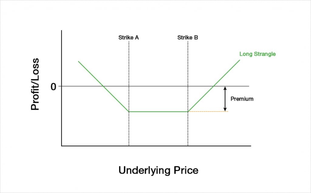
The maximum loss of the long strangle is capped at the premium paid. This maximum loss will occur if the underlying price is anywhere between strikes A and B at expiry. Compared to the long straddle, we have a wider range where we can take a maximum loss, however the total premium paid will be lower, so the magnitude of the maximum loss is smaller.
The maximum profit is uncapped in both directions (other than by the underlying price reaching zero to the downside), and in dollar terms the payoff is symmetrical. We have had to purchase both the put and the call, meaning a larger net debit has been paid than if we had chosen a direction by only purchasing one of the options. However, the debit will be smaller than the debit we would have paid to establish a long straddle instead. The trade off there being that the underlying price needs to move further for a long strangle to make a profit, than it would have for a long straddle.
If we hold the long strangle until expiry with no further adjustments, it is simply a bet that the underlying price will have moved outside of a certain range. This range is determined by our two breakeven points. In dollar terms, the breakeven points can be calculated as:
First Breakeven = Strike price A – Premium
Second Breakeven = Strike price B + Premium
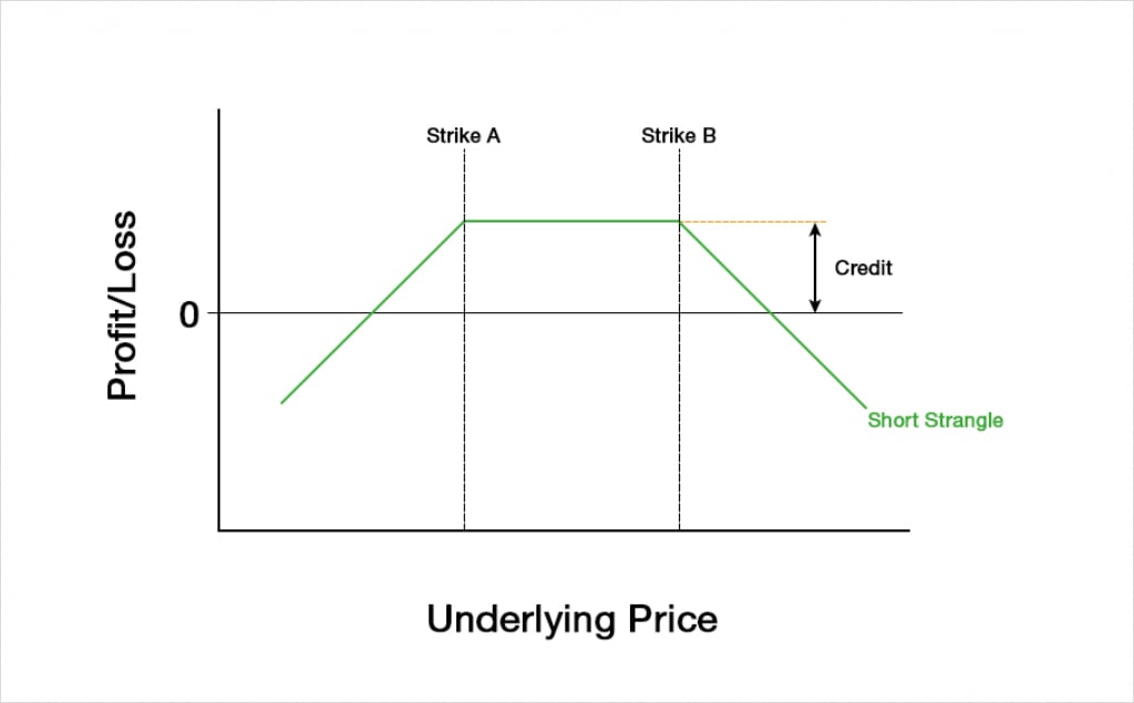
These breakeven points are shared by the short strangle, but the profit and loss are of course flipped. This means the short strangle has a fixed maximum profit of the credit received, with unlimited risk on each side. The attractive property of a strangle from the seller’s point of view is that they can profit from a wider price range than they could with a short straddle. The maximum profit will be smaller though.
The Greeks
For the following section on the PNL and the Greeks, we will focus on the values for the long strangle. To get the values for the short strangle, we just need to multiply by minus one. This just changes the sign of any value, and as always, any gain for the buyer is a loss for the seller, and vice versa.
We can add our Greek values for the put at strike A to the values for the call at strike B, and this will give us the total Greek values for the long strangle.
To analyse how the Greeks behave we will use the following figures:
Underlying price: $100
Time to expiry: 50 days
Interest rate: 0
Implied volatility: 60%
Strike A: $80
Strike B: $120
Profit and loss
With these parameters the $80/$120 strangle will initially cost us about $4.44. The payoff chart looks like this.
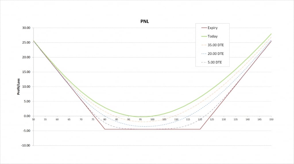
The maximum loss is capped at the premium paid, which is $4.44. The maximum loss occurs when the underlying price is anywhere between our two strikes of $80 and $120 at expiry.
To the downside, the maximum profit is only capped if the underlying price reaches zero, and to the upside the maximum profit is completely uncapped. The further the price moves in either direction the more money we make at expiry.
There are two breakeven prices, one to the upside and one to the downside. The one to the downside is calculated by subtracting the total premium paid from the strike price of the put, which gives us:
$80 – $4.44 = $75.56
The breakeven price to the upside is calculated by adding the total premium paid to the strike price of the call, which gives us:
$120 + $4.44 = $124.44
The seller of the strangle has these same breakeven points, but the seller has a fixed maximum profit and unlimited risk.
Delta
The long strangle can have either a positive or negative delta. The sign of the delta depends on where the underlying price is relative to the strike price.
This chart shows the delta of the long strangle, with the x axis being the underlying price. The extra lines also show how the delta will evolve as time passes.
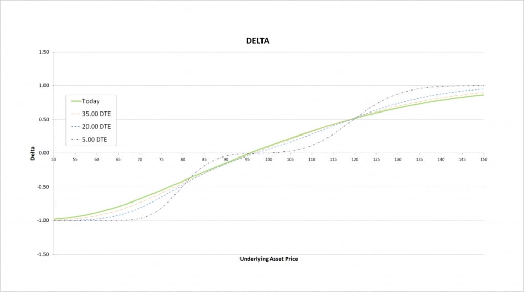
When the underlying price is between our two strikes, the positive delta gained from the call and the negative delta gained from the put largely cancel each other out. The total delta for the long strangle is therefore small when the underlying price is in the middle of our strikes. The wider the range between our two strikes, the more the delta will vary over that range.
When the underlying price decreases, the negative delta from the put option increases in magnitude, whereas the positive delta from the call decreases in magnitude. Both of these have the effect of making our total delta increasingly negative as the underlying price decreases. The more the underlying price decreases, the more negative our delta becomes, meaning we effectively get more short the underlying as the price decreases. Eventually the delta of the deep OTM call approaches 0, while the delta of the deep ITM put approaches -1. This means our total delta approaches -1 as the underlying price continues to decrease.
Conversely, when the underlying price increases, the negative delta from the put decreases in magnitude, whereas the positive delta from the call increases in magnitude. Both of these have the effect of making our total delta increasingly positive as the underlying price increases. The more the underlying price increases, the more positive our delta becomes, meaning we effectively get more long the underlying as the price increases. Eventually the delta of the deep OTM put approaches 0, while the delta of the deep ITM call approaches 1. This means our total delta approaches 1 as the underlying price continues to increase.
So by being long a strangle, we are effectively speculating that the market will trend. The more the market does trend, the more the long strangle will make.
As time passes, if the underlying price is below the strike of our put option, our delta will tend towards -1, and if the underlying price is above the strike price of our call option, our delta will tend towards 1. Unlike with the straddle that we looked at previously though, there is a gap between the put strike and the call strike. This means when the underlying price is between the two strikes, both options are OTM. As we approach expiration, this will cause our delta to approach zero instead. When the underlying price is between the strikes of $80 and $120, the delta approaches zero as time passes.
Gamma
As we move from left to right on the delta chart, the delta of the long strangle is always increasing. This means the gamma is always positive.
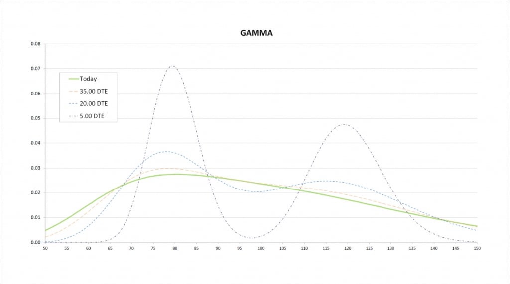
The steeper the delta line, the more extreme the gamma is. With 50 days remaining, the delta line is steepest when we are relatively close to the strike price of the put, so this is where gamma peaks.
The gamma of the long strangle changes shape as time passes. We are long both options, but the strike prices are relatively far apart. This eventually leads to two very distinct peaks in the gamma. The peaks occur at each of our strike prices, and they get taller and thinner the closer we get to expiry.
Vega
We are long both a put and a call. Both of these options have positive vega, so our total vega for the long strangle is always positive, and always greater than for either of the two individual options.

The buyer of any option has a positive vega. The magnitude of this vega is greatest when the option is close to the money, and as time passes, the magnitude decreases no matter where the underlying price is in relation to the strike price.
Similar to what we saw with the gamma, as time passes the two peaks from having vega concentrated around our two strikes become clearer. As we get closer to expiry, vega peaks when the underlying price is close to either of our strikes, and is close to zero everywhere else.
As the vega is always positive, the long stangle always benefits from an increase in implied volatility, and suffers from a decrease in implied volatility. If all else remains equal and implied volatility increases, both the put and the call will increase in value, resulting in a double gain for our long strangle.
Theta
Time is against us when we hold a long strangle. All long options have negative theta, meaning they lose value as time passes. With a long strangle we are long a put and a call, both of which will lose value as time passes. It’s also only possible for a maximum of one of them to be ITM at expiry so at least one of them is guaranteed to lose all of its value by expiry, and there is also a range where both will expire worthless.
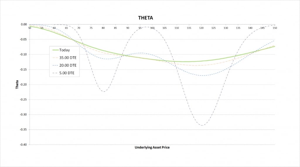
The magnitude of the theta is greatest when the underlying price is close to the strike price of the call option. As time passes, the theta concentrates around each of the two strikes, and the magnitude of the peaks increases.
Inverse option contracts
A long strangle consists of a long put and a long call. The same is true when using the inverse option contracts on Deribit.
This chart shows the bitcoin payoff at expiry of a long strangle using the bitcoin options on Deribit. In this example we’ve purchased one call option with a strike price of $55,000, and purchased one put option also with a strike price of $45,000. We pay a total of 0.08BTC for the long strangle.
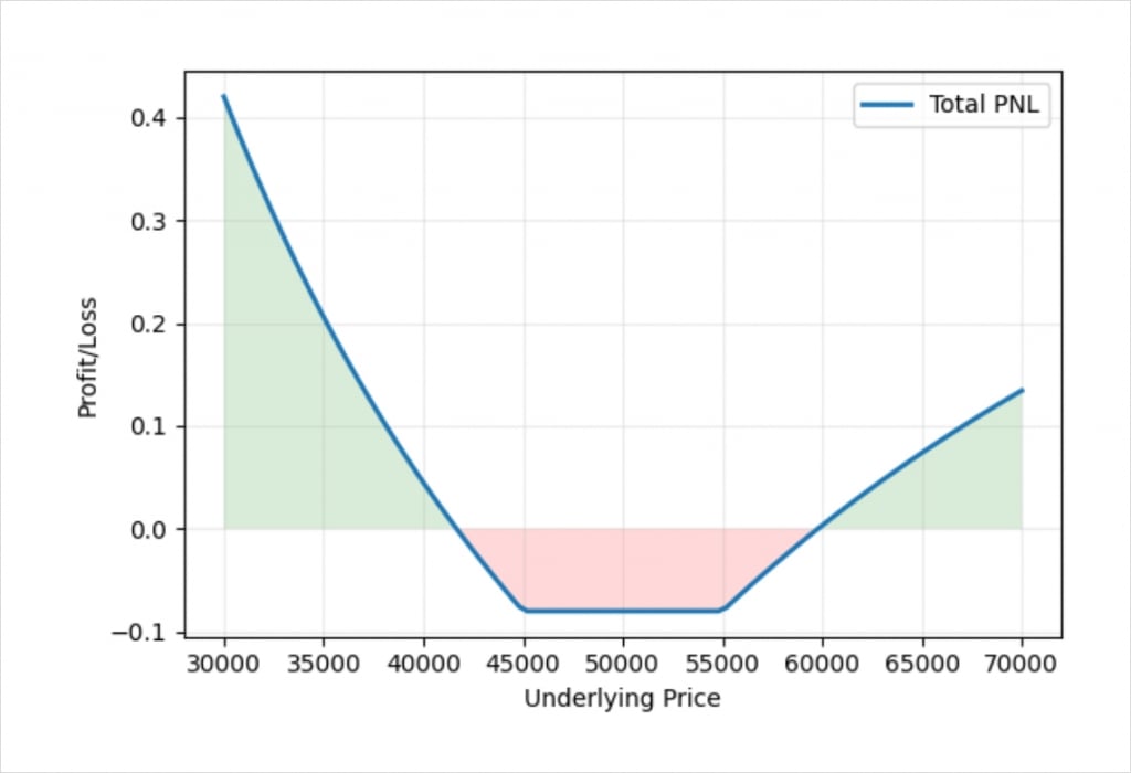
The shape of the profit/loss in bitcoin terms is similar to the profit/loss in dollar terms that we saw earlier. Due to the nature of payoffs with inverse contracts, the line is curved instead of straight, and we can also see that if the underlying price decreases, we make more bitcoin than for an equivalent increase in price. This is due to how much bitcoin it takes to pay a fixed amount of dollars when the underlying price is different.
Even without calculating them precisely, we can see that this also leads to the breakeven points not being symmetrical around our strangle. If the underlying price is $5,000 above our call strike at expiry, this will be close to a breakeven trade. However, if the underlying price is $5,000 below the strike price of our put strike at expiry, this will result in a modest profit for the long strangle in bitcoin terms.
The dollar value of the strangle is exactly the same in both cases, but the bitcoin value is very different. This is due to the difference in the underlying bitcoin price at expiry. The dollar profit/loss chart is still perfectly symmetrical, but the bitcoin profit/loss chart is not.
Strangles
Strangles are similar to straddles, but instead of being fixed to a single strike price, the strangle creates a wider range that we are speculating on. This results in a reduction in initial cost, but wider breakeven points. The peak values for the Greeks are also smaller in magnitude for the strangle than for the straddle, however the underlying price range where the Greeks remain significant is also wider for the strangle.
We have looked at the long strangle here, but you should be comfortable converting everything we have said so that it applies to short strangles instead. If the long strangle has positive gamma and vega, and negative theta, then it should be clear that a short strangle has negative gamma and vega, and positive theta.
A long strangle has a fixed risk and unlimited potential profit, so a short strangle has a fixed maximum profit, and unlimited risk. The values are simply the opposite, and this is true in both dollar and bitcoin terms.