

In this lecture we will be looking at back spreads and front spreads, both with call options. A back spread is the opposite of a front spread. That is, for us to execute a back spread position, the trader on the other side of the trade would be by definition executing a front spread, and vice versa (assuming both legs are traded as a single position).
You may also see these strategies referred to as ratio spreads. They consist of two different options, and the reason they are known as ratio spreads is that, unlike with something like a vertical spread, the ratio of the position size we use for each of the two options is not 1:1. You may see ratio spreads talked about as a 1×2 (one by two), a 1×3 (one by three), or a 2×3 (two by three) for example. While other ratios can be used, 1:2 is common, and is what we will use in this lecture.
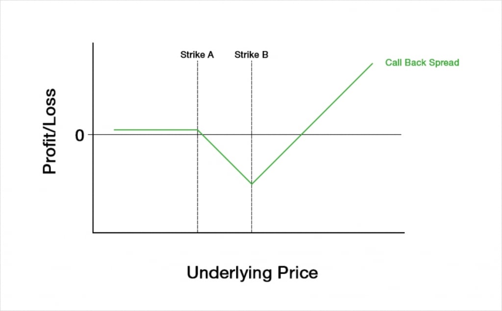
A call back spread is a bullish strategy, and therefore gives us a positive delta. The call back spread is constructed by:
-Selling a call option with strike price A
-Purchasing 2 call options with strike price B, where B > A
The underlying price will typically be at or below A.
The call front spread is just the opposite of this. So we would instead buy a call at strike A, and sell 2 calls at strike B.
In both cases, both of the calls have the same expiry date, and the underlying price is typically somewhere at or below A.
Ideally we would collect a small credit when establishing the position, however this won’t always be the case so we may pay a small debit instead. If we do manage to establish the call back spread for a small credit, this gives us a payoff chart that looks like this.
The maximum loss of the call back spread is fixed, but can still be large. The maximum loss is equal to:
Maximum loss = Strike B – Strike A + X
Where X is the net amount we pay to establish the position. If we receive a credit instead then this number (X) will be negative, and will have the effect of decreasing the magnitude of the maximum loss.
The maximum loss occurs when the underlying price is precisely equal to strike B at expiry.
The maximum profit is unlimited to the upside, but the underlying price needs to increase significantly for a large profit to be made at expiry. One of the attractive features of a back spread is that if we are completely wrong on the direction, our risk is minimal, and we may even make a small profit if the strategy is established for a net credit. When established for a credit, we also make a small profit if the underlying price is below strike A at expiry.
When established for a net credit we also have two breakeven points. In dollar terms, the breakeven points can be calculated as:
First Breakeven = Strike A + Credit received
Second Breakeven = Strike B + (Strike B – Strike A + X)
Where X is the net amount we pay to establish the position. The Second part of the calculation in brackets here is, as you may have noticed, equal to the maximum loss we mentioned earlier.
If instead of receiving a net credit, we pay a net debit to establish the position, then we only have the second breakeven point. The first breakeven point will no longer exist as the PNL line no longer crosses the x axis into profit to the downside.
These breakeven points are shared by the opposing call front spread, but the profit and loss are of course flipped around the x axis.
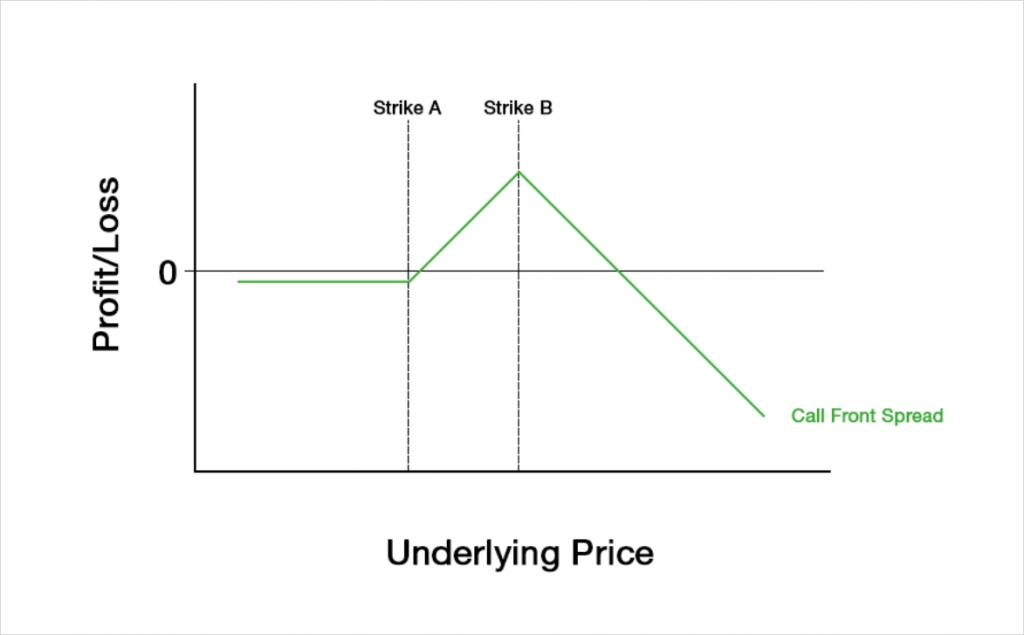
We’ve just flipped our example PNL around the x axis here so the front spread has been established for a net debit, but ideally we would also want to establish a front spread for a net credit if possible. For the front spread, this will be easier when OTM options are being priced significantly higher in implied volatility terms than the ATM options. When this is the case, the 2 options that we are selling that are further OTM will be priced higher in IV terms, so we should collect a larger premium for them than if the volatility smile were flatter.
If the volatility smile subsequently flattens off, this can lead to an immediate profit for the front spread, without the underlying price even having to move. More generally, with a front spread, as we are short 2 options and only long 1, a decrease in implied volatility will be good for us in most situations. Conversely for the back spread, as we are long 2 options and only short 1, an increase in implied volatility will be good for us in most situations.
The Greeks
For the following sections on the PNL and the Greeks, we will focus on the values for the call back spread. To get the values for the call front spread, we just need to multiply by minus one. This just changes the sign of any value, and as always, any gain for the buyer is a loss for the sell, and vice versa.
We can add our Greek values for the call at strike A to the values for the calls at strike B, and this will give us the total Greek values for the call back spread.
To analyse how the Greeks behave we will use the following figures:
Underlying price: $100
Time to expiry: 50 days
Interest rate: 0
Implied volatility: 60%
Strike A: $110
Strike B: $120
Profit and loss
With these parameters the $110/$120 1×2 call back spread will initially cost us about $0.49. The payoff chart looks like this.
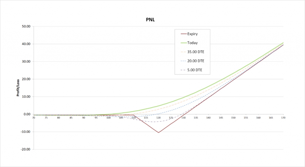
The maximum loss is capped by this formula that we gave earlier. Where X is the net amount we pay to establish the position.
= Strike B – Strike A + X
= 120 – 110 + 0.49
= $10.49
This maximum loss occurs when the underlying price is precisely at strike B ($120) at expiry.
As we paid a net debit for the call back spread, we will also make a small loss if the underlying price is below strike A ($110) at expiry. This loss is limited to the debit paid of $0.49.
If we had instead established the spread for a net credit, our profit to the downside would be limited to the credit collected. Whether we pay a debit or collect a credit though, the potential profit to the upside is unlimited.
As we have paid a net debit for the spread, we only have one breakeven point. The breakeven point is calculated as:
= Strike B + (Strike B – Strike A + X)
= 120 + (120 – 110 + 0.49)
= 120 + 10.49
= $130.49
The seller on the other side of the trade, who has the corresponding front spread, has the same breakeven point, but they have a fixed maximum profit and unlimited risk to the upside.
Delta
The call back spread is a bullish strategy, and as such the delta is mostly (but not always) positive.
This chart shows the delta of the call back spread, with the x axis being the underlying price. The extra lines also show how the delta will evolve as time passes.
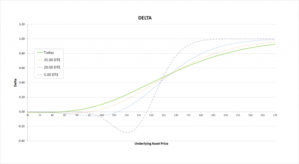
When both of the calls are far OTM, our delta is very close to zero. The delta then increases as the underlying price increases. When the position is first placed, the delta looks remarkably similar to that of a single long call option. This is logical as we are net long one call option.
As time passes though, the delta line dips into negative values when the underlying price is just below our short strike A. By looking at the profit/loss chart we can see why this is the case. As we get closer to expiry, the risk is that the underlying price will end up close to our long strike B. As expiry approaches, if the underlying price is sitting close to our short strike A, there is not much time left for the price to rally hard, so a small increase in price just makes it more likely we are going to suffer a bigger loss, hence the negative delta in this area.
Gamma
When the position is first opened, as we move from left to right on the delta chart, the delta of the call back spread is always increasing. This means the gamma is always positive.
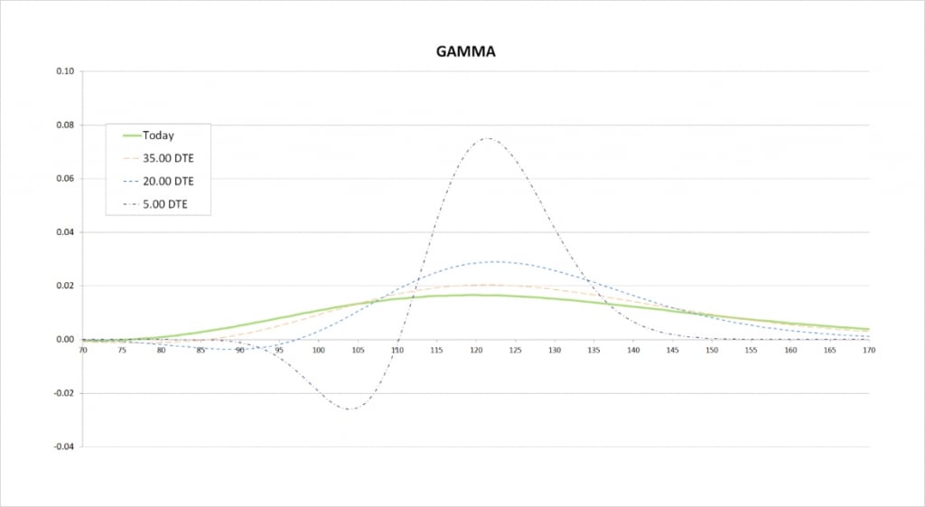
The steeper the delta line, the more extreme the gamma is. The delta line is steepest when we are relatively close to the long strike of $120, so this is where gamma peaks.
As time passes, we get the dip in the delta close to the short strike that we talked about. This creates two extremes on the gamma chart. One negative peak just below our short strike, and one positive peak close to our long strike. We are long twice as many options at the $120 strike as we are short options at the $110 strike, so the positive peak we see in gamma at the $120 strike is of a greater magnitude.
This gamma is telling us that most of the time our delta increases as the underlying price increases. The exception to this is when the underlying price is just below our short strike where our delta can decrease if the underlying price only increases by a small amount. This effect gets stronger the closer we get to expiry.
Vega
We are short one call, but long another with double the size, so we are net long one call. This means on the whole we gain from an increase in implied volatility, and so have a positive vega.
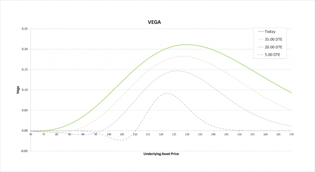
As with the delta and gamma, our vega position looks similar to that of a long call option at first. An increase in implied volatility will increase the value of our short call (which is bad for us), but will also increase the value of our 2 long calls, which more than makes up for it. As time passes though, we have negative vega when the underlying price is just below our short strike.
As a reminder, as with everything we’re covering here, if we were instead holding the front spread instead of the back spread, all of these values would be flipped around the x axis. So the front spread will have mostly negative vega, meaning it benefits when implied volatility decreases instead.
Theta
We are net long options, so time is against us. Our theta is mostly negative with the call back spread.
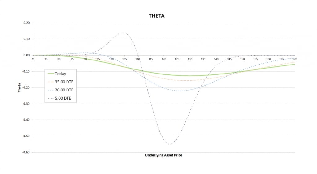
As time passes the negative theta becomes larger in magnitude when we are close to our long strike. We don’t want to be sitting in the belly of the spread as we get closer to expiry. When the options expire, this is where we would suffer the largest loss, and as we get close to expiry this is where we will bleed time value the fastest.
If the price is resting close to our long strike for too long, we may wish to close the back spread early to avoid the increasing pace of losses while price sits there.
Inverse option contracts
The call back spread looks very similar when using inverse contracts as well.
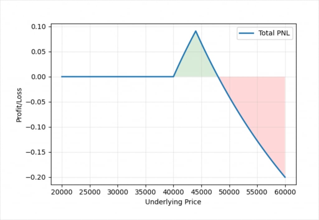
This chart shows the bitcoin payoff at expiry of a call back spread using the bitcoin options on Deribit. In this example we’ve sold one call option with a strike price of $40,000, and purchased two call options with a strike price of $44,000. We collect 0.1 BTC for the $40,000 call, and pay 0.05 each for the $44,000 calls, and therefore establish the position for zero credit or debit.
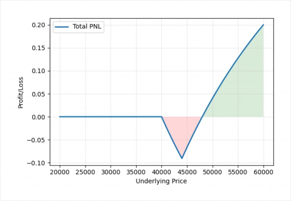
The shape of the profit/loss in bitcoin terms is relatively similar to the profit/loss in dollar terms that we saw earlier, just with the usual curve to the lines we see with inverse contracts.
We still have a fixed risk, but much like when long a single bitcoin call option, the profit is capped at 1 BTC. In fact the profit is capped at 1 BTC minus the net debit (or plus the net credit) we paid to establish the position. As this example was established for a net of zero though, the maximum profit is capped at 1 BTC.
If we change the range of the chart to include higher prices, we can more clearly see the diminishing returns in bitcoin terms as the underlying price increases.
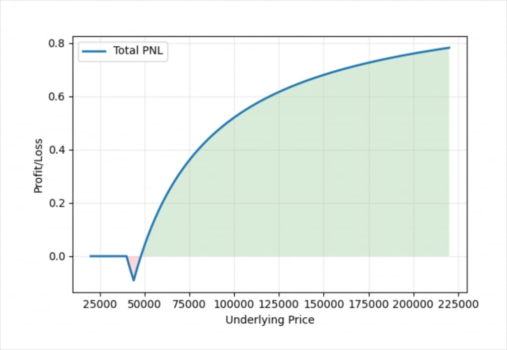
If we were to keep extending the right side of the chart, the profit line would get closer and closer to 1, without ever quite reaching it.
For the trader on the other side of this trade, who is holding the front spread, this profit/loss is of course flipped around the x axis.
When are back spreads and front spreads attractive?
Call back spreads will be most attractive when we are extremely bullish on an asset that has the potential to make large moves in price. If we are completely wrong on the direction, we will not lose much if anything, but when we are correct and the price increases significantly, we can make large profits.
We will most easily be able to establish the back spread for free or even for a net credit, when the IV for OTM calls is similar or lower than the IV for ATM calls.
Conversely, call front spreads will be most attractive when we are most confident that there will not be a large increase in the underlying price. For call front spreads, ideally we would like the IV for OTM calls to be much higher than the IV for ATM calls. This way we can purchase a single ATM call for relatively cheap, while collecting inflated premiums for the 2 OTM calls that we sell. This will make it easier for us to collect a net credit while establishing the position.