

The first option strategy we’re going to study is the bull call spread. As the name suggests, a bull call spread is a bullish strategy, and therefore has a positive delta.
The strategy is constructed by:
– Purchasing a call option at strike price A.
– Selling a different call option with a higher strike price B, but the same expiry date.
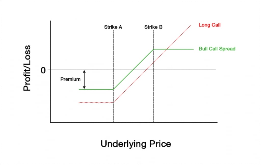
The option with strike A is purchased, meaning a debit is paid, however the option with strike B is sold, meaning a credit is received. As strike A is lower than strike B, the call option with strike A will be more expensive than the call option with strike B, meaning we will have to pay a net debit overall. This will lead to a payoff chart that looks something like this at expiry:
It’s worth noting that for the moment we are talking in dollar terms here. We will come onto how this chart looks for the inverse option contracts on Deribit shortly.
As you can see towards the left side of the chart, much like when only purchasing a call option, a bull call spread is a fixed risk strategy. The maximum loss is limited to the net premium paid to establish the position. This occurs at expiry when the underlying price is lower than the strike of the purchased option with strike A.
Unlike when only purchasing a call option though, the potential profit of a bull call spread is also capped. This can be seen on the right side of the chart, where the P&L line flattens off again. This occurs at expiry when the underlying price is higher than the strike of the sold option with strike B.
Buying a call option gives a trader a fixed risk and unlimited potential reward. By adding in the short leg at strike B, the bull call spread has capped the potential profit, meaning it’s now a fixed risk, and fixed reward strategy. Obviously this change by itself is less desirable for the trader, so how are they compensated? Because the call at strike B is sold, the trader collects a credit for this leg, and although this credit will be smaller than the debit paid for the call at strike A, the total cost has been reduced. This reduction in cost brings the breakeven price lower, meaning that the underlying price has to move less before the trader starts to show a profit.
Compared to only buying a call, a bull call spread gives the trader a reduced cost and a lower breakeven price, but also caps their potential profit. They pay less up front, but once the price moves above strike B, the trader no longer benefits from any further increases (at expiry at least).
The Greeks
In sections 8 to 11, we covered the option Greeks. We gave an introduction to delta, gamma, vega, and theta. In each of those sections we mentioned that it’s possible to sum the Greeks for the individual legs to get the total values for the whole position. For example, to get the total delta for the bull spread, if we assume a position size of one for each leg, we can simply subtract the delta for the call at strike B from the delta of the call at strike A.
Bull call spread delta = Delta at strike A – Delta at strike B
The reason we are subtracting the delta of the call at strike B instead of adding it, is because we are short this option. Our position size is -1, so we multiply the delta by -1 when calculating our delta for this option.
In section 12, we will look at how the Greeks for each of the strategies behave. We will study how they are affected by changes in the underlying price, and how they evolve as time passes.
To analyse how the Greeks behave we will need to assign some figures to each of the parameters that we enter into Black Scholes calculations. These calculations are what give us the Greek values. For today’s example of a bull call spread we will assume the following parameters:
Underlying price: $100
Time to expiry: 50 days
Interest rate: 0
Implied volatility: 60%
Strike A: $110
Strike B: $115
Although we covered in section 7 that the implied volatility will usually vary across different strike prices, to keep things simple we will assume the same implied volatility figure for each strike. We will do this for every strategy in this section.
Profit and loss
With these parameters the $110/$115 bull call spread will initially cost about $1.31 to buy. The payoff chart looks like this.
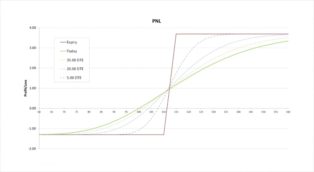
The maximum profit is capped at the difference between the two strikes minus the net premium paid. The difference between the long strike and the short strike is $5, and the net premium paid is $1.31, so the maximum profit for this trade is:
$5 – $1.31 = $3.69
The maximum profit occurs when the underlying price is at or above the short strike of $115 at expiry. The maximum loss of $1.31 occurs when the underlying price is at or below the long strike of $110 at expiry. The breakeven can be calculated by adding the net premium to the strike price of the long option. In this case it gives us:
$110 + $1.31 = $111.31
Delta
As we know from section 8, delta tells us how much an option’s value is expected to change due to an increase in the underlying price of $1. When we have a position consisting of several options, our total delta tells us how much the whole position’s value is expected to change due to an increase in the underlying price of $1.
As a bull call spread is a bullish trade that benefits from an increase in the underlying price, the total delta will be positive. We are long the $110 call, which has a positive delta. We are also short the $115 call which by itself gives us some negative delta. However, because the delta of the $110 call will always be larger than the delta of the higher strike $115 call, our total delta for a bull call spread will always be positive.
This chart shows the delta of the bull call spread, with the x axis being the underlying price. The extra lines also show how the delta will evolve as time passes.
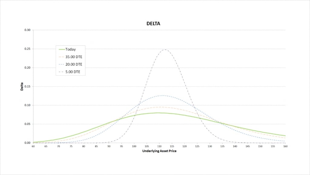
The first thing you may notice, is that unlike with a single call option, where the delta continues to increase as the underlying price increases, the delta of the bull call spread peaks once the long call is in the money. The delta is also considerably lower than 1. Remember, both call options will always have a delta of between 0 and 1, and also that the delta of the $110 strike will always be higher than the delta of the $115 strike. As we are short the $115 strike, this means that the total delta for the bull call spread must also be between 0 and 1. Due to the parameters chosen, they currently largely cancel each other out though no matter where the underlying price moves, leading to a delta of considerably less than 1.
As time passes, the peak delta gets higher, and the price range where there is any significant delta reduces significantly. As we come into expiry this effect accelerates. The peak delta can be seen when the long call is ITM, but the short call is still OTM. This is because as days to expiry (DTE) approaches 0, the delta of ITM calls approaches 1 and the delta of OTM calls approaches 0.
To briefly summarise the delta characteristics of the bull call spread, the delta is always positive, and is highest when the underlying price is between the two strikes.
Gamma
Gamma is the rate of change of delta as the underlying price changes. In other words it tells us how steep the line is on the delta chart. As we move from left to right on the delta chart, whenever the delta is increasing, this means the gamma is positive. Whenever the delta is decreasing, this means the gamma is negative. The steeper the line, the more extreme the gamma is. Remembering this can help understand what we are looking at when we look at this gamma chart.
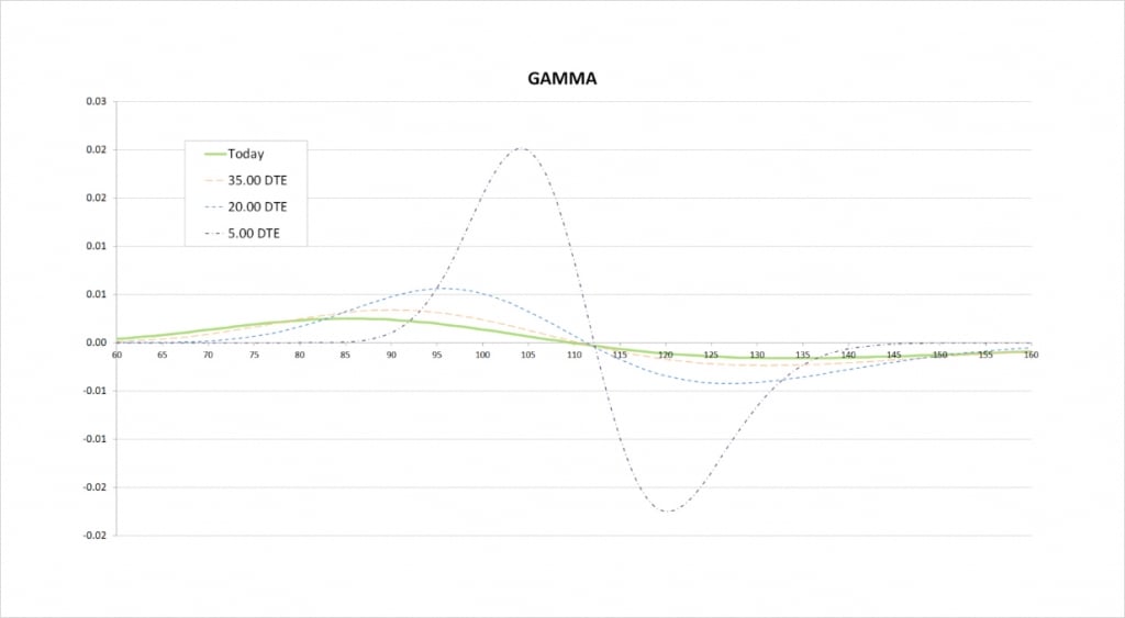
For the current values of delta with 50 days remaining until expiry, we see that delta increases slowly, peaks around the price of our long strike of $110, then decreases slowly. On the gamma chart this is shown by gamma starting positive, then crossing the x axis at about the $110 strike, and then turning negative.
When we get much closer to expiry, the price range where there is any significant delta is much narrower, and delta changes much quicker. On the gamma chart this results in a narrower price range for significant gamma, and much more extreme values of gamma due to the more rapid changes in delta. The less time until the options expire, the closer the peaks in gamma will be to the strike prices of the options.
With the gamma, it’s interesting to note that we don’t just have one peak/trough on the chart like we do with delta, we now have two. Gamma is most extreme when delta is changing at the fastest rate. This happens both when the delta is increasing quickly and when the delta is decreasing quickly. So one peak in delta leads to two extremes in gamma, one on the way up, and one on the way down.
Vega
Vega tells us how an option’s value will change due to a change in implied volatility. An increase in implied volatility will increase the value of both puts and calls. Long options therefore have positive vega, and short options have negative vega. We are long one call and short another call here, so we will always have one leg with positive vega and one leg with negative vega.
The magnitude of an option’s vega will depend where the underlying price currently is relative to the strike price of each option, with options that are close to the money typically having the greatest vega. Whether our bull call spread has negative or positive vega, will therefore depend on where the underlying price is relative to the strikes.
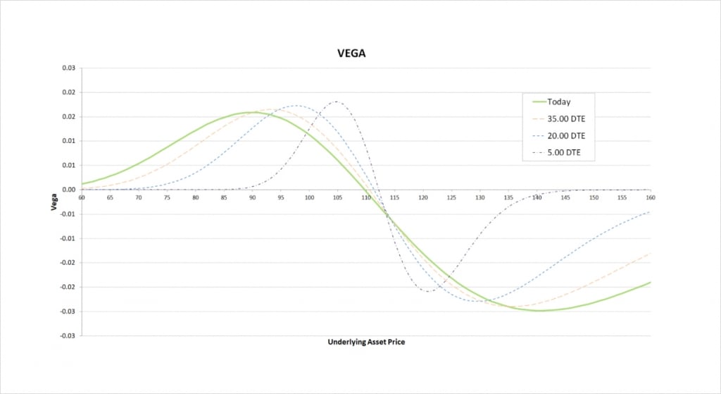
We are long the $110 call which gives us some positive vega, and we are short the $115 call which gives us some negative vega. To the left of the chart, we can see that because the $110 call is closer to the money, the positive vega we gain from this option outweighs the negative vega from the $115 call.
As we move to the point where both options are relatively close to the money, their vegas approximately cancel each other out, giving the bull call spread a very small vega value. The precise point where vega is zero varies a little depending on how much time is left until the options expire.
Once we get to the right side of the chart, with the underlying price above both strikes, the $115 strike is closer to the money. This leads to the negative vega of the $115 strike outweighing the smaller positive vega we have from the $110 strike. The vega of the bull call spread is therefore negative here.
The less time is left until the options expire, the closer the underlying price has to be to our strike prices for the spread to have any significant vega. As we come into expiry, if both options are either far ITM or far OTM, then vega will be close to zero.
Theta
Theta tells us the rate an option is currently losing value as time passes. Long options lose value as time passes, resulting in a negative value for theta. For short options, the loss of value represents a gain, resulting in a positive value for theta. We are long one call and short another call, so we will always have one negative theta and one positive theta.
The magnitude of an option’s theta will depend on where the underlying price currently is relative to the strike price of each option, with options that are close to the money typically having the greatest theta. So, whether our bull call spread has negative or positive theta depends on where the underlying price is relative to the strikes.
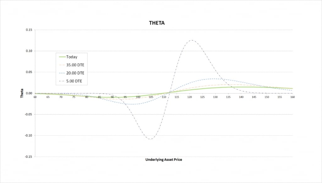
The theta chart looks quite similar to the gamma chart, if it were multiplied by -1.
To the left of the chart, we can see that because the $110 call is closer to the money, the negative theta we have from this option outweighs the positive theta from the $115 call.
As we move to the point where both options are relatively close to the money, their thetas largely cancel each other out, giving the bull call spread a very small theta value.
Once we get to the right side of the chart, with the underlying price above both strikes, the $115 strike is closer to the money. This leads to the positive theta of the $115 strike outweighing the smaller negative theta we have from the $110 strike. The theta of the bull call spread is therefore positive here.
The less time is left until the options expire, the closer the underlying price has to be to our strike prices for the spread to have any significant theta. As we come into expiry, if both options are either far ITM or far OTM, then theta will be close to zero. You may remember from lecture 9.4, that far ITM or far OTM options have little extrinsic value remaining as expiry approaches, therefore they have very little value to lose to time decay.
Theta of the long call
If we compare the theta of the spread to the theta of just the long $110 call, we can see one effect that using a bull call spread has had on our Greeks compared to just longing a call.
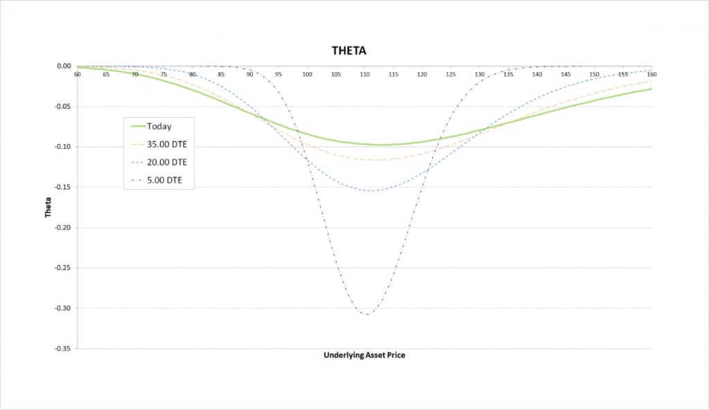
If we had just purchased the $110 call, our theta with 50 days remaining could be as much as -0.10, meaning the position could lose up to $0.10 a day just due to the passage of time. With the bull call spread though, the theta with 50 days remaining is never any more than about -0.01, meaning the position will only lose up to $0.01 a day as time passes.
Spreads often have this effect of reducing the magnitude of certain greeks compared to single option strategies. In certain circumstances this can be very attractive. In this example, if you were initially worried that the $110 call by itself may be a little overpriced and so you may be losing too much value to theta every day while you wait for the underlying price to move, you may consider the bull call spread more attractive. Particularly if you believe the $115 call is even more overpriced.
Inverse option contracts
When we discussed the payoff chart of the bull call spread earlier, we worked in dollar terms. We showed the profit and loss values assuming everything is paid/received in dollars. However, the inverse contracts on Deribit use the cryptocurrency itself as collateral. The profit/loss is still calculated in dollars first, but is then paid/received in the cryptocurrency, not in dollars. This means it is useful to know what the payoff looks like when measured in this cryptocurrency.
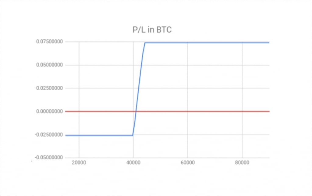
This chart shows the bitcoin payoff at expiry of a bull call spread using the bitcoin options on Deribit. In this example we’ve purchased one call option with a strike price of $40,000, and sold one call option with a strike price of $44,000. The $40,000 call costs us 0.06 BTC, and we receive a 0.04 BTC credit for the $44,000 call.
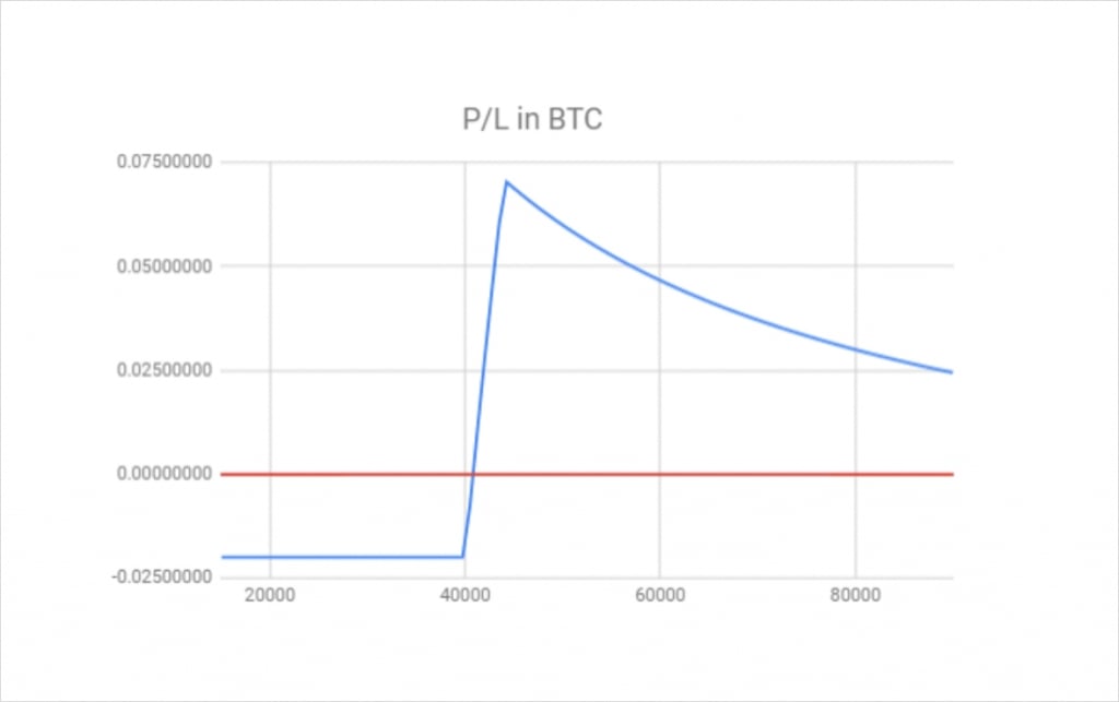
If the price expires below our short strike of $44,000, the chart looks similar to the dollar example earlier. The risk is fixed to the net debit of 0.02 BTC that we paid to place the spread. The profit line then increases between the two strikes, however, although it looks almost straight here, the increase is not actually linear. Once we get above the short strike of $44,000, it becomes clear that something different is happening.
As the size of our long leg and short leg is the same here (both a size of 1), the dollar value of the maximum profit is still fixed, as it was in the dollar only example earlier. The reason the maximum profit is not straight on this BTC payoff chart though, is because as the underlying price of bitcoin increases, the amount of bitcoin required to pay this fixed amount of dollars is reduced.
The difference between the long strike of $40,000 and the short strike of $44,000, is of course $4,000. When the underlying price at expiration is above $44,000, we therefore expect to receive this difference of $4,000 as the intrinsic value of our bull call spread. How much bitcoin it takes to pay us the equivalent of $4,000 though, depends on what the bitcoin price is at the time our payout is calculated at expiry.
If the price of bitcoin at expiry is exactly $44,000, then we will receive about 0.0909 BTC, which is equivalent to $4,000 at the time. Our profit will be this amount minus the 0.02 BTC we initially paid for the spread. However, if the price of bitcoin at expiry is $50,000 instead, we will only receive 0.08 BTC, which is still equivalent to $4,000 at the time. So the dollar value remains the same at $4,000, but the bitcoin amount has changed due to the different underlying price.
For more details and examples of how the profit and loss for cryptocurrency call and put options is calculated, refer back to lectures 4.2 and 6.2 respectively.
Defining fixed risk/reward with inverse contracts
For those that care more about the bitcoin value of their account than the dollar value, it is possible to fix the reward in bitcoin terms instead of dollar terms. We can achieve this with an adjustment to the position sizing between the two legs.
If we adjust our position sizing such that the ratio between the size of each of our two legs is the inverse of the ratio between the two strike prices, we achieve something that looks like this.
The ratio of the strike prices is:
40,000 : 44,000
This is equal to:
1 : 1.1
If we simply invert this, we get a position sizing ratio that will set the reward to a fixed amount of bitcoin. This gives us a position sizing ratio of:
1.1 : 1
So if we buy the $40,000 call with a position size of 1.1, and sell the $44,000 call with a position size of 1, we get a position that is fixed risk and fixed reward in bitcoin terms, as desired.
There are a couple of issues to note when doing this though. Firstly, in this case, as we have had to increase the size of our long leg, this means the net cost of placing the spread has increased. Our risk has increased from 0.02 BTC to 0.026 BTC.
It’s also worth noting that with smaller position sizes, it may not always be possible to set this ratio up perfectly. Due to minimum trade sizes, we may not always be able to perfectly adjust one leg to the necessary ratio and still remain within our personal risk limits. However, as long as we can get close it will behave very similarly.
Portfolio margin on Deribit
Now that we are beginning to use strategies that contain multiple legs, it’s well worth mentioning how options are margined on Deribit. The standard margin system on Deribit calculates the margin for each of your legs separately, and then adds them all together to calculate your total margin requirements. For futures positions or single option positions this works fine. However, when you start to trade option strategies that have multiple legs that partially or entirely hedge each other, margin requirements can be lowered significantly by switching to the Deribit portfolio margin system. The portfolio margin system looks at how the entire portfolio of positions in the account would perform with changing market conditions. If the positions hedge each other, as they do with a bull call spread for example, this will be taken into account and will reduce the total margin requirements in many cases.
For more information on this margining system, it is well worth going through this lesson on the Deribit blog here.