

If you understood the previous strategy of a bull call spread, this lecture on a bear call spread should be incredibly simple to understand, because a bear call spread is the exact opposite of a bull call spread.
In the previous lecture we were looking at the strategy from the perspective of the buyer of the bull call spread, but the trader on the other side of that trade, i.e. the person who sold us the bull call spread, was by definition entering a bear call spread with the same parameters.
The strategy is constructed by:
– Selling a call option at strike price A.
– Purchasing a different call option with a higher strike price B, but the same expiry date.
As with the previous bull call spread, we are buying one call and selling another call. With the bull call spread, we were buying the lower of the two strikes. However, with the bear call spread we are selling the lower of the two strikes.
As the name suggests, despite still using only call options, a bear call spread is a bearish strategy, and therefore has a negative delta.
The option with strike A is sold, meaning a credit is collected, and the option with strike B is purchased, meaning a debit is paid. As strike A is lower than strike B, the call option with strike A will be more expensive than the call option with strike B, meaning we will collect a net credit overall. This will lead to a payoff chart that looks something like this at expiry:
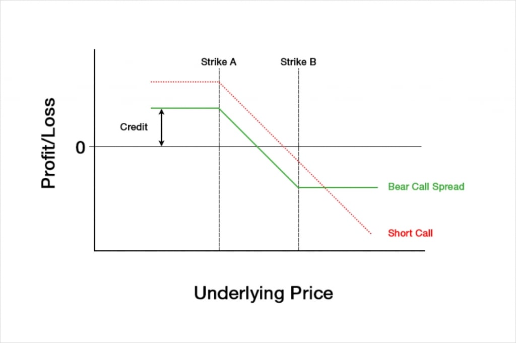
Just like when only selling a call option, the maximum profit for a bear call spread is capped. The maximum profit is limited to the net credit collected. This occurs at expiry when the underlying price is lower than strike A.
Unlike when only selling a call option though, the potential loss of a bear call spread is also capped. This can be seen on the right side of the chart, where the P&L line flattens off again. This occurs at expiry when the underlying price is higher than strike B.
Selling a call option gives a trader a fixed potential profit but unlimited risk. By adding in the long leg at strike B, the bear call spread has capped the risk, meaning it’s now a fixed risk, fixed reward strategy. This change by itself is very desirable for the trader, so what is the catch? Because the call at strike B is bought, the trader pays a debit for this leg, and although this debit will be smaller than the credit collected for the call at strike A, the total collected has been reduced. This reduction in credit brings the breakeven price lower, meaning that the underlying price has to increase less before the trader starts to make a loss.
Compared to only selling a call, a bear call spread gives the trader a smaller potential profit, but it also caps their risk. They collect a smaller net credit, but once the price moves above strike B, the trader is no longer hurt by any further increases (at expiry at least).
The Greeks
As we’ve already learned, it’s possible to sum the Greeks for the individual legs to get the total values for the whole position. So, we can simply add our Greek values for the call at strike A to the values for the call at strike B, and this will give us the total Greek values for the bear call spread.
To analyse how the Greeks behave we will need to assign some figures to each of the Black Scholes parameters. For today’s example of a bear call spread we will assume the following parameters:
Underlying price: $100
Time to expiry: 50 days
Interest rate: 0
Implied volatility: 60%
Strike A: $110
Strike B: $115
These are exactly the same as the values we used in the previous lecture. This will help illustrate that the bear call spread is indeed the exact opposite of the bull call spread.
Profit and loss
With these parameters the $110/$115 bear call spread will initially give us a credit of about $1.31. The payoff chart looks like this.
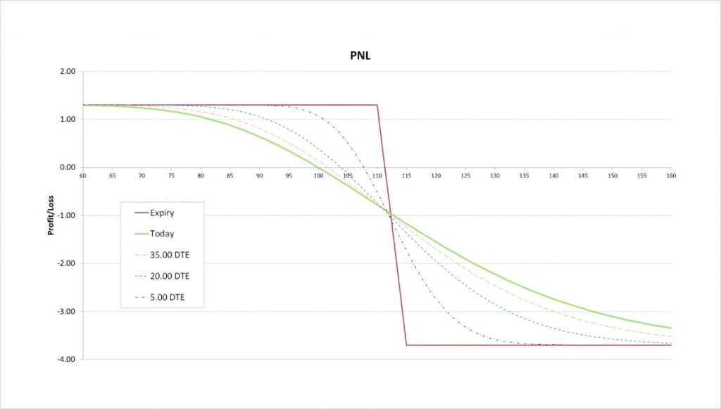
The maximum profit is capped at the net premium collected, which is $1.31. This maximum profit occurs when the underlying price is at or below the short strike of $110 at expiry.
The maximum loss is capped at the difference between the two strikes minus the net credit received. The difference between the long strike and the short strike is $5, and the net credit is $1.31, so the maximum loss for this trade is:
$5 – $1.31 = $3.69
Notice that this is the same as the maximum profit for the bull call spread in the previous lecture. In any trade, a loss for one side is a profit for the other side, and vice versa.
(Note: We are of course ignoring trading fees here for simplicity)
The maximum loss occurs when the underlying price is at or above the long strike of $115 at expiry. It is this long strike at $115 that is capping our maximum loss compared to just being short the $110 call. We are effectively short the underlying between $110 and $115, but once $115 is breached to the upside, we are effectively flat again.
The breakeven can be calculated by adding the net credit collected to the strike price of the short option. This gives us:
$110 + $1.31 = $111.31
This is exactly the same breakeven price as the bull call spread in the previous lecture.
Delta
As a bear call spread is a bearish trade that benefits from a decrease in the underlying price, the total delta will be negative. We are short the $110 call, which gives us some negative delta. We are also long the $115 call which gives us some positive delta. Because the delta of the $110 call will always be larger than the delta of the higher strike $115 call though, our total delta for a bear call spread will always be negative.
This chart shows the delta of the bear call spread, with the x axis being the underlying price. The extra lines also show how the delta will evolve as time passes.
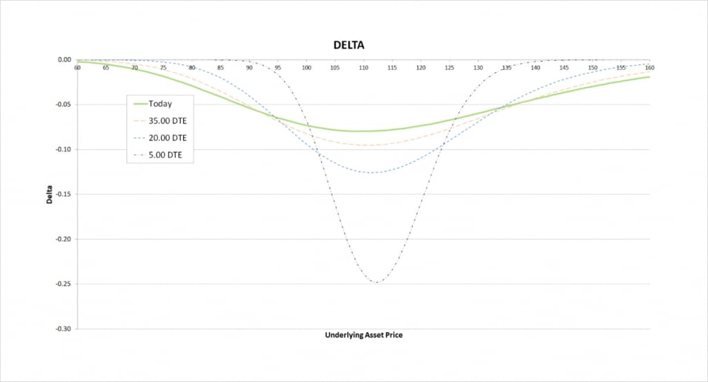
The delta of the bear call spread peaks once the short call is in the money. Both call options will always have a delta of between 0 and 1, and the delta of the $110 strike will always be greater than the delta of the $115 strike. As we are short the $110 strike, this means that the total delta for the bear call spread must also be between 0 and -1. Due to the parameters chosen, they currently mostly cancel each other out though no matter where the underlying price moves, leading to a delta of considerably less magnitude than -1.
As time passes, the peak delta becomes more extreme, and the price range where there is any significant delta reduces significantly. As we come into expiry this effect accelerates. The peak delta can be seen when the short call at $110 is ITM, but the long call at $115 is still OTM. This is because as days to expiry (DTE) approaches 0, the delta of ITM calls approaches 1 and the delta of OTM calls approaches 0. Therefore, when the underlying price is between the two strikes as we are getting close to expiry, the delta our ITM short call is giving us is approaching -1, and the delta our OTM long call is giving us is approaching 0. This means our total delta is approaching -1.
The delta for the bear call spread then, is always negative, and peaks when the underlying price is between the two strikes.
Gamma
As always, as we move from left to right on the delta chart, whenever the delta is increasing, this means the gamma is positive. Whenever the delta is decreasing, this means the gamma is negative. The steeper the line, the more extreme the gamma is. It is useful to remember this when studying gamma charts.
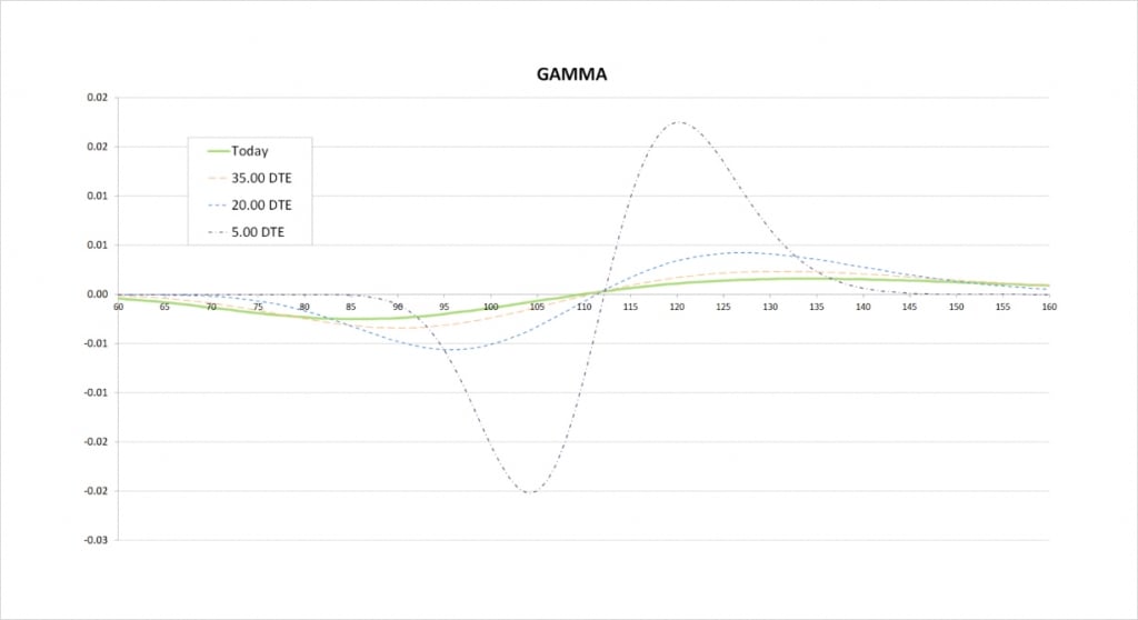
For the current values of delta with 50 days remaining until expiry, we see that delta decreases slowly, peaks around the price of our short strike of $110, then increases slowly. On the gamma chart this is shown by gamma starting negative, then crossing the x axis at about the $110 strike, and then turning positive.
When we get much closer to expiry, the price range where there is any significant delta is much narrower, and delta changes much quicker. On the gamma chart this results in a narrower price range for significant gamma, and much more extreme values of gamma due to the more rapid changes in delta. The less time until the options expire, the closer the peaks in gamma will be to the strike prices of the options.
Gamma is most extreme when delta is changing at the fastest rate. This happens both when the delta is decreasing quickly and when the delta is increasing quickly. So one peak in delta leads to two extremes in gamma, one on the way down, and one on the way up.
Vega
With a bear call spread, we are long one call and short another call, so we will always have one positive vega and one negative vega.
The magnitude of an option’s vega depends on where the underlying price currently is relative to the strike price of the option. Whether our bear call spread has negative or positive vega will therefore depend on where the underlying price is relative to the strikes.
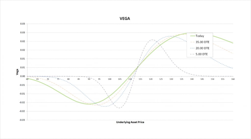
We are short the $110 call which gives us some negative vega, and we are long the $115 call which gives us some positive vega. To the left of the chart, we can see that because the $110 call is closer to the money, the negative vega we gain from this option outweighs the positive vega from the $115 call.
As we move to the point where both options are relatively close to the money, their vegas mostly cancel each other out, giving the bear call spread a very small vega value. The precise point where vega is zero varies a little depending on how much time is left until the options expire.
Once we get to the right side of the chart, with the underlying price above both strikes, the $115 strike is closer to the money. This leads to the positive vega of the $115 strike outweighing the smaller negative vega we have from the $110 strike. The vega of the bear call spread is therefore positive here.
The less time is left until the options expire, the closer the underlying price has to be to our strike prices for the spread to have any significant vega. As we come into expiry, if both options are either far ITM or far OTM, then vega will be close to zero.
Theta
We are long one call and short another call, so we will always have one negative theta and one positive theta. Whether our bear call spread has negative or positive theta depends on where the underlying price is relative to the strikes.
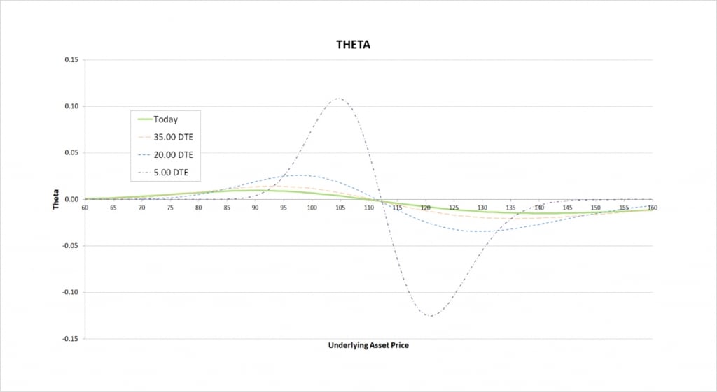
To the left of the theta chart, we can see that because the $110 call is closer to the money, the positive theta we have from this option outweighs the negative theta from the $115 call.
As we move to the point where both options are relatively close to the money, their thetas mostly cancel each other out, giving the bear call spread a very small theta value.
Once we get to the right side of the chart, with the underlying price above both strikes, the $115 strike is closer to the money. This leads to the negative theta of the $115 strike outweighing the smaller positive theta we have from the $110 strike. The theta of the bear call spread is therefore negative here.
The less time is left until the options expire, the closer the underlying price has to be to our strike prices for the spread to have any significant theta. As we come into expiry, if both options are either far ITM or far OTM, then theta will be close to zero. Far ITM or far OTM options have little extrinsic value remaining as expiry approaches, therefore they have very little value to lose to time decay.
Inverse option contracts
When we discussed the payoff chart of the bear call spread earlier, we worked in dollar terms. We showed the profit and loss values assuming everything is paid/received in dollars. However, the inverse contracts on Deribit use the cryptocurrency itself as collateral. The profit/loss is calculated in dollars first, but is then paid/received in the cryptocurrency, not in dollars. This means it is useful to know what the payoff looks like when measured in this cryptocurrency.
This chart shows the bitcoin payoff at expiry of a bear call spread using the bitcoin options on Deribit. In this example we’ve sold one call option with a strike price of $40,000, and purchased one call option with a strike price of $44,000. We receive a credit of 0.06 BTC for the $40,000 call, and we pay 0.04 BTC for the $44,000 call.
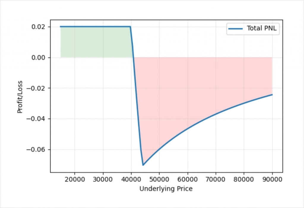
If the price expires below our short strike of $44,000, the chart looks similar to the dollar example earlier. The maximum profit is fixed to the net credit of 0.02 BTC that we received for the spread. The profit line then decreases between the two strikes, however, although it looks almost straight here, the increase is not actually linear. Once we get above the long strike of $44,000, it becomes clear that the payoff line is not linear.
As the size of our long leg and short leg are the same here (both a size of 1), the dollar value of the maximum loss is still fixed, as it was in the dollar example earlier. The reason the maximum loss is not straight on this BTC payoff chart though, is because as the underlying price of bitcoin increases, the amount of bitcoin required to pay this fixed amount of dollars is reduced.
The difference between the short strike of $40,000 and the long strike of $44,000, is $4,000. When the underlying price at expiration is above $44,000, we therefore expect to have to pay out this difference of $4,000 as the intrinsic value of our bear call spread. How much bitcoin it takes us to pay the equivalent of $4,000 though, depends on exactly what the bitcoin price is at the time.
If the price of bitcoin at expiry is exactly $44,000, then we will need to pay about 0.0909 BTC, which is equivalent to $4,000 at the time. Our total loss will be this amount minus the 0.02 BTC we initially collected for the spread. However, if the price of bitcoin at expiry is $100,000 instead, we will only need to pay 0.04 BTC, which is still equivalent to $4,000 at the time. So the dollar value remains the same at $4,000, but the bitcoin amount has changed significantly due to the different underlying price.
Defining fixed risk/reward with inverse contracts
Just like we were able to fix the bitcoin reward of the bull call spread in the previous lecture, it is possible to fix the risk of the bear call spread in bitcoin terms instead of dollar terms. We can achieve this with an adjustment to the position sizing between the two legs.
If we adjust our position sizing so that the ratio between the size of each of our two legs is the inverse of the ratio between the two strike prices, we achieve something that looks like this.
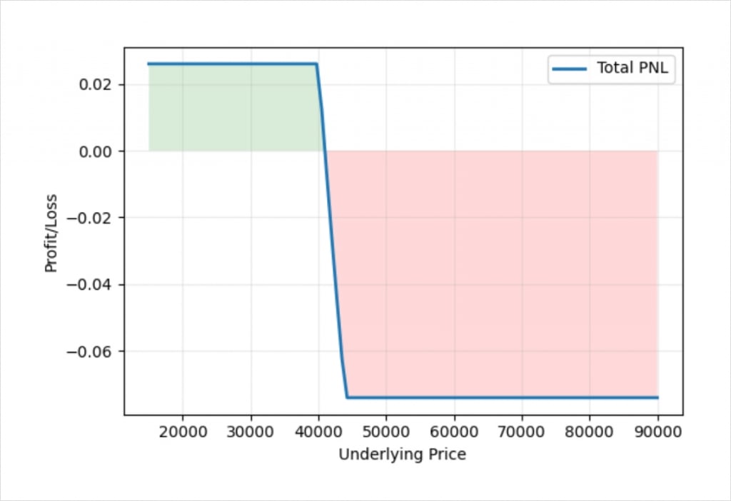
As before, the ratio of the strike prices is:
40,000 : 44,000
This is equal to:
1 : 1.1
If we invert this, we get a position sizing ratio that will set the risk to a fixed amount of bitcoin. This gives us a position sizing ratio of:
1.1 : 1
So if we sell the $40,000 call with a position size of 1.1, and buy the $44,000 call with a position size of 1, we get a position that is fixed risk and fixed reward in bitcoin terms, as desired.
In bitcoin terms, if we execute the bear call spread at a 1:1 ratio, although the risk is not a fixed amount, it is already capped. So we don’t need to worry about unlimited risk in bitcoin terms. In fact, once the long strike is breached, we actually lose less BTC if the underlying price continues to rally. Eventually we may even turn a profit, once the amount of bitcoin required to pay the fixed amount of dollars is smaller than the fixed amount of bitcoin that we initially collected for the spread. If we’re happy with this characteristic, and the credit collected, then we can leave the ratio alone. However, if we do choose to fix the risk, this allows us to collect a larger net credit initially, without increasing our maximum loss at all.