

In the previous two lectures, we’ve looked at a bull spread and a bear spread, both executed using calls. However, it’s possible to execute both spreads with put options instead and get a position with a very similar payoff chart, though they do differ when we look at the inverse contracts. Whether they are executed with calls or puts, both are also often referred to as vertical spreads.
In the following two lectures we will look first at a bear put spread, and then at a bull put spread. The first four lectures in this section are going to be a little repetitive, but this will give traders who are newer to options the opportunity to get comfortable with the difference between each side of a multi-leg option position. As we move further into this section, we will assume readers are comfortable with inferring one side of a strategy from the other. If you’re already comfortable with vertical spreads, you may want to double check you’re aware of how inverse contracts affect the payoffs for put spreads, but then you can probably skip to lecture 12.6 if you prefer.
A bear put spread is a bearish strategy, and therefore gives us a negative delta. The strategy is constructed by:
-Purchasing a put option at strike price B.
-Selling a different put option with a lower strike price A, but the same expiry date.
The option with strike B is purchased, meaning a debit is paid, and the option with strike A is sold, meaning a credit is collected. As strike A is lower than strike B, the put option with strike B will be more expensive than the put option with strike A, meaning we will pay a net debit overall. This will lead to a payoff chart that looks something like this at expiry:
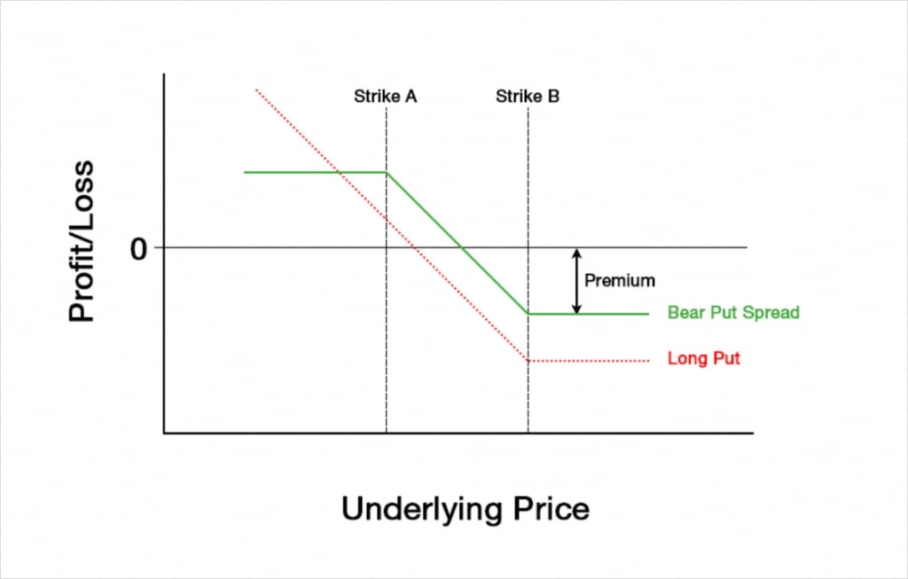
Just like when only purchasing a put option, the risk is capped. The maximum loss is limited to the net debit paid. This occurs at expiry when the underlying price is higher than the strike of the purchased option with strike B.
Unlike when purchasing a put option though, the potential profit of a bear put spread is also capped. This can be seen on the left side of the chart, where the P&L line flattens off again. This occurs at expiry when the underlying price is lower than the strike of the sold put with strike A.
Buying a put option gives a trader a fixed risk and (almost) unlimited potential reward. By adding in the short leg at strike A, the bear put spread has capped the potential profit, meaning it’s now a fixed risk, fixed reward strategy. Obviously this change by itself is less desirable for the trader, so how are they compensated? Because the put at strike A is sold, the trader collects a credit for this leg, and although this credit will be smaller than the debit paid for the put at strike B, the total cost has been reduced. This reduction in cost brings the breakeven price higher, meaning that the underlying price has to move less before the trader starts to show a profit.
Compared to only buying a put, a bear put spread gives the trader a reduced cost, but also caps their potential profit. They pay less up front, but once the price moves below strike A, the trader no longer benefits from any further decreases in the underlying price (at expiry at least).
The Greeks
We can add our Greek values for the put at strike A to the values for the put at strike B, and this will give us the total Greek values for the bear put spread.
To analyse how the Greeks behave we will need to assign some figures to each of the Black Scholes parameters. For today’s example of a bear put spread we will assume the following parameters:
Underlying price: $100
Time to expiry: 50 days
Interest rate: 0
Implied volatility: 60%
Strike A: $90
Strike B: $85
The strikes chosen make both puts OTM, similar to how both calls were OTM in lectures 12.2 and 12.3.
Profit and loss
With these parameters the $90/$85 bear put spread will initially cost about $1.56 to buy. The payoff chart looks like this.
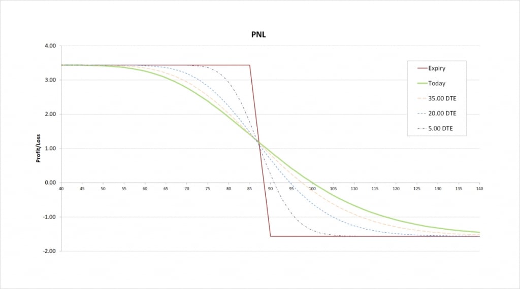
The payoff of the bear put spread looks similar to that of the bear call spread, and indeed the charts for the Greeks also look similar, which we will look at shortly.
The maximum profit is capped at the difference between the two strikes minus the net premium paid. The difference between the long strike of $90 and the short strike of $85 is $5, and the net premium paid is $1.56, so the maximum profit for this trade is:
$5 – $1.56 = $3.44
This maximum profit occurs when the underlying price is at or below the short strike of $85 at expiry.
The maximum loss of $1.56 occurs when the underlying price is at or above the long strike of $90 at expiry.
The breakeven can be calculated by subtracting the net premium from the strike price of the long option. In this case it gives us:
$90 + $1.56 = $88.44
Delta
As a bear put spread is a bearish trade that benefits from a decrease in the underlying price, the total delta will be negative. We are long the $90 put, which gives us some negative delta. We are also short the $85 put which gives us some positive delta. Because the delta of the $90 put will always be of a larger magnitude than the delta of the lower strike $85 put though, our total delta for a bear put spread will always be negative.
This chart shows the delta of the bear put spread, with the x axis being the underlying price. The extra lines also show how the delta will evolve as time passes.
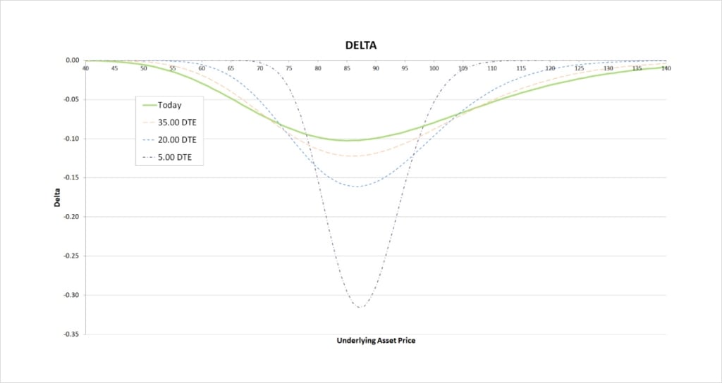
The delta of the bear put spread peaks once the short put is in the money. Both put options will always have a delta of between 0 and -1, and the delta of the $90 strike will always be more negative than the delta of the $85 strike. As we are long the $90 strike, this means that the total delta for the bear put spread must also be between 0 and -1. Due to the parameters chosen, they currently mostly cancel each other out though no matter where the underlying price moves, leading to a delta of considerably less magnitude than -1.
As time passes, the peak delta becomes more extreme, and the price range where there is any significant delta reduces significantly. As we come into expiry this effect accelerates. The peak delta can be seen when the long put at $90 is ITM, but the short put at $85 is still OTM. This is because as days to expiry (DTE) approaches 0, the delta of ITM puts approaches -1 and the delta of OTM puts approaches 0. Therefore, when the underlying price is between the two strikes as we are getting close to expiry, the delta our ITM long put is giving us is approaching -1, and the delta our OTM short put is giving us is approaching 0. This means our total delta is approaching -1.
The delta for the bear put spread then, is always negative, and peaks when the underlying price is between the two strikes. You may also notice that the shape of the delta chart for the bear put spread is almost identical to the delta chart for the bear call spread.
Gamma
As always, as we move from left to right on the delta chart, whenever the delta is increasing, this means the gamma is positive. Whenever the delta is decreasing, this means the gamma is negative. The steeper the line on the delta chart, the more extreme the gamma is.
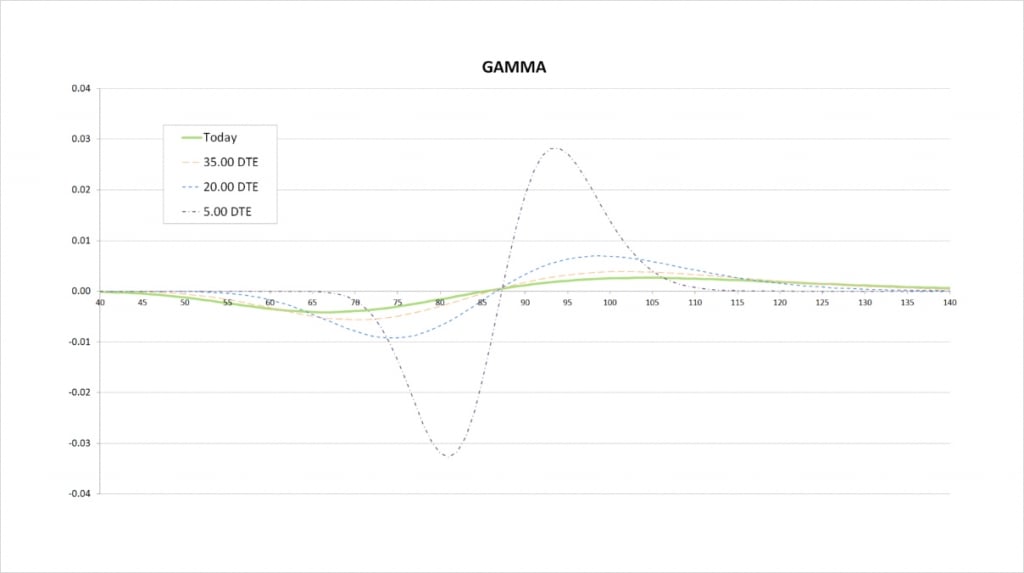
For the current values of delta with 50 days remaining until expiry, we see that delta decreases slowly, peaks around the price of our short strike of $85, then increases slowly. On the gamma chart this is shown by gamma starting negative, then crossing the x axis at about the $85 strike, and then turning positive.
When we get much closer to expiry, the price range where there is any significant delta is much narrower, and delta changes much quicker. On the gamma chart this results in a narrower price range for significant gamma, and much more extreme values of gamma due to the more rapid changes in delta. The less time until the options expire, the closer the peaks in gamma will be to the strike prices of the options.
Gamma is most extreme when delta is changing at the fastest rate. This happens both when the delta is decreasing quickly and when the delta is increasing quickly. So one peak in delta leads to two extremes in gamma, one on the way down, and one on the way up.
This gamma chart for the bear put spread is again very similar to that of the bear call spread.
Vega
We are long one put and short another put here, so, as with the delta, we will always have one positive vega and one negative vega.
The magnitude of an option’s vega depends on where the underlying price currently is relative to the strike price of the option. Whether our bear put spread has negative or positive vega will therefore depend on where the underlying price is relative to the strikes.
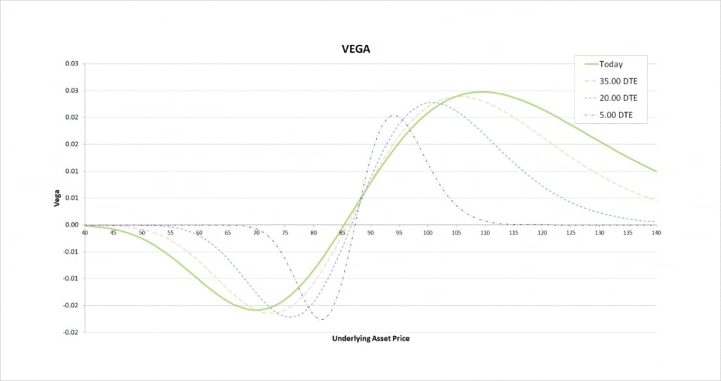
We are long the $90 put which gives us some positive vega, and we are short the $85 put which gives us some negative vega. To the left of the chart, we can see that because the $85 put is closer to the money, the negative vega we gain from this option outweighs the positive vega from the $90 put.
As we move to the point where both options are relatively close to the money, their vegas largely cancel each other out, giving the bear put spread a very small vega value.
Once we get to the right side of the chart, with the underlying price above both strikes, the $90 strike is closer to the money. This leads to the positive vega from being long the $90 strike outweighing the smaller negative vega we have from being short the $85 strike. The vega of the bear put spread is therefore positive here.
The less time is left until the options expire, the closer the underlying price has to be to our strike prices for the spread to have any significant vega. As we come into expiry, if both options are either far ITM or far OTM, then vega will be close to zero.
Theta
We are long one put and short another put, so we will always have one negative theta and one positive theta. Whether our bear put spread has negative or positive theta depends on where the underlying price is relative to the strikes.
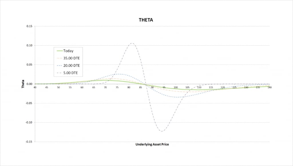
To the left of the theta chart, we can see that because the $85 put is closer to the money, the positive theta we have from this option outweighs the negative theta from the $90 put.
As we move to the point where both options are relatively close to the money, their thetas largely cancel each other out, giving the bear put spread a very small theta value.
Once we get to the right side of the chart, with the underlying price above both strikes, the $90 strike is closer to the money. This leads to the negative theta from being long the $90 strike outweighing the smaller positive theta we have from being short the $85 strike. The theta of the bear put spread is therefore negative here.
The less time is left until the options expire, the closer the underlying price has to be to our strike prices for the spread to have any significant theta. As we come into expiry, if both options are either far ITM or far OTM, then theta will be close to zero.
Inverse option contracts
So far, everything we’ve looked at for the bear put spread, from the payoff in dollars to the shape of the Greek charts, has been extremely similar to what we saw in lecture 12.3 for the bear call spread.
When we look at how the payoff charts behave for inverse contracts, we see an important difference between how puts and calls behave.
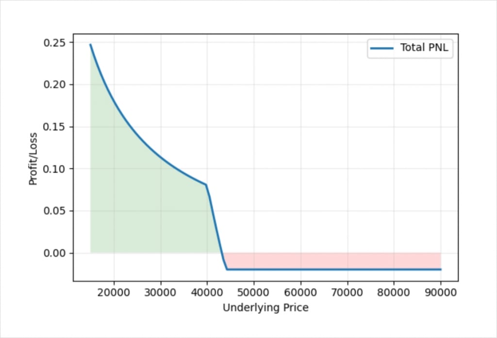
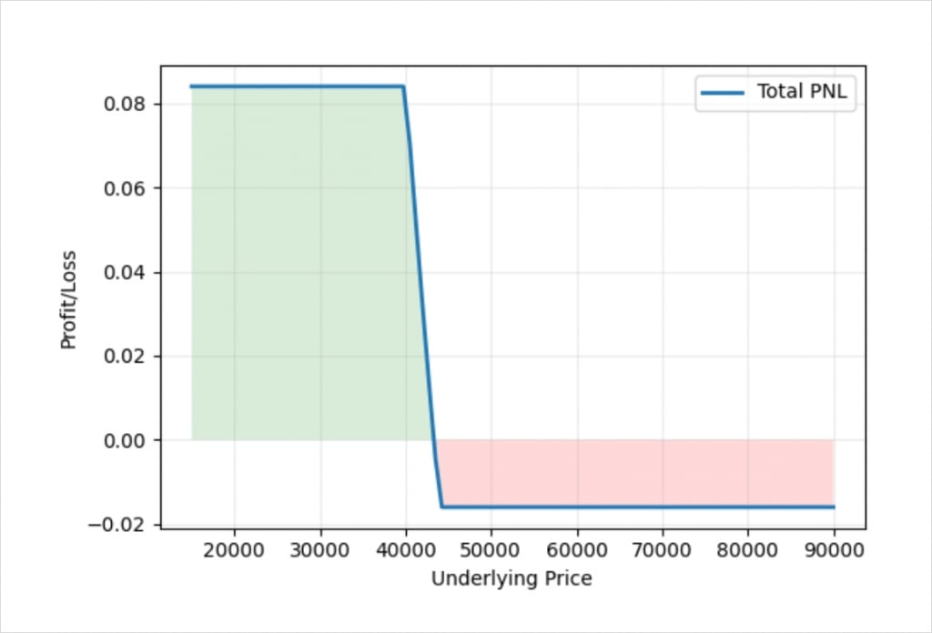
This chart shows the bitcoin payoff at expiry of a bear put spread using the bitcoin options on Deribit. In this example we’ve purchased one put option with a strike price of $44,000, and sold one put option with a strike price of $40,000. We pay a debit of 0.06 BTC for the $44,000 put, and we receive a 0.04 BTC credit for the $40,000 put.
Let’s compare this to the payoff of the bear call spread on bitcoin that we looked at in lecture 12.3.
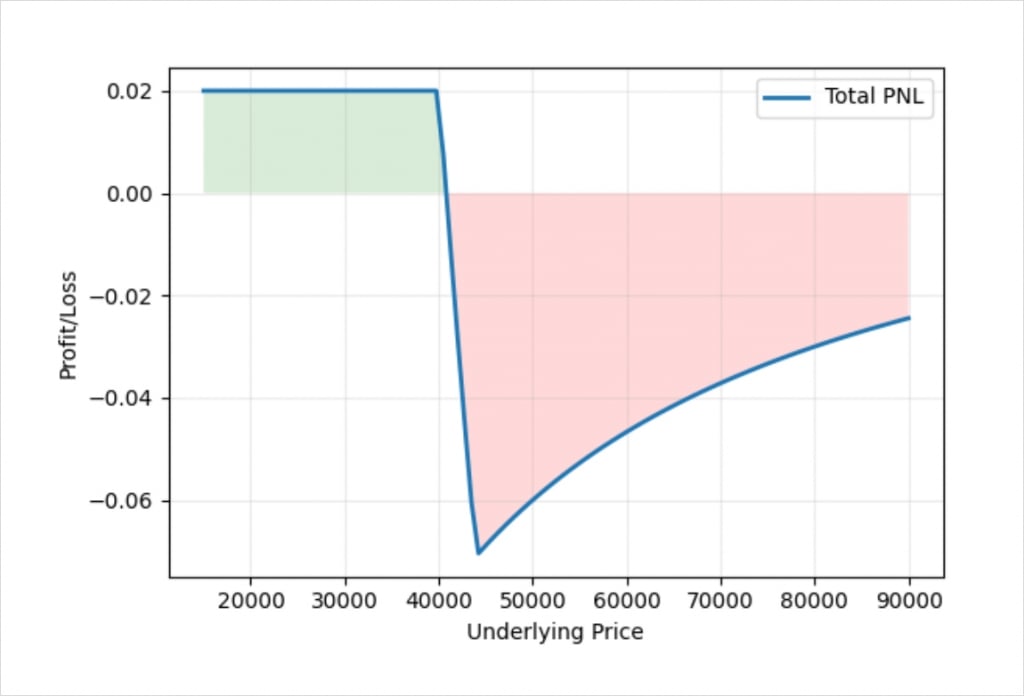
As we can see, there is a noticeable difference between these two payoff charts. Especially when compared to how similar a bear call spread and a bear put spread look in dollar terms.
If the price expires below our short put strike of $40,000, we see that the profit in bitcoin continues to increase as the bitcoin price decreases. As the size of our long leg and short leg are the same here (both a size of 1), the dollar value of the maximum profit is still fixed, as it was in the dollar example earlier. The reason the maximum profit is not straight on the BTC payoff chart for the bear put spread though, is because as the underlying price of bitcoin decreases, the amount of bitcoin required to pay this fixed amount of dollars is increased.
For the bear call spread, the profit here is fixed. This is because for a bear call spread, when the underlying price expires below both strikes, this means that they are both OTM. There is no intrinsic value to calculate, and our profit is fixed to the amount of bitcoin that was initially collected for the spread. For the bear put spread though, when the underlying price expires below both strikes, this means that they are both ITM. This means there is an intrinsic value to calculate, and this value is first calculated in dollars, but then converted to and paid in bitcoin.
As an example of how this results in different BTC values for the spread, it takes twice as much bitcoin to pay us the $4,000 value of the spread when the bitcoin price is at $20,000 (0.2 BTC), as it does when the bitcoin price is at $40,000 (0.1 BTC).
Defining fixed risk/reward with inverse contracts
It is still possible to fix both the risk and reward for the bear put spread in bitcoin terms. In this instance we receive more bitcoin as the bitcoin price continues to decrease, so we may wish to leave the spread in this state. Our risk remains fixed, so it’s not exactly a problem that we make more bitcoin as the price falls. However, there is a reason we may wish to define the reward as well as the risk.
The fact that our profit measured in bitcoin continues to increase as the price of bitcoin decreases, means we have room to sell more of the $40,000 strike puts. In doing so we will collect a larger credit for the short leg.
If we adjust our position sizing so that the ratio between the size of each of our two legs is the inverse of the ratio between the two strike prices, we achieve something that looks like this.
The ratio of the strike prices is:
40,000 : 44,000
Which is equal to:
1 : 1.1
If we invert this, we get a position sizing ratio that will set the reward to a fixed amount of bitcoin. This gives us a position sizing ratio of:
1.1 : 1
So if we sell the $40,000 put with a position size of 1.1, and buy the $44,000 put with a position size of 1, we get a position that is fixed risk and fixed reward in bitcoin terms, as desired.
Earlier we stated the prices of the $40,000 and $44,000 puts as 0.04 and 0.06 BTC respectively. When we execute the spread with a 1 : 1 ratio, this results in us paying a net debit of 0.02 BTC. However when we execute the spread with a 1.1 : 1 ratio, we collect an extra credit of 0.004 BTC. This reduces our net debit for the spread to 0.016 BTC. So by adjusting the relative size of the two legs, we’ve reduced our maximum risk, but capped the maximum profit in BTC terms. Bear in mind this also means that once our short strike of $40,000 is breached to the downside, the lower the bitcoin price is at expiry, the less this fixed amount of bitcoin will be worth in dollar terms.
Puts or calls
We’ve shown that a bear call spread is very similar to a bear put spread, and indeed the same is true of bullish vertical spreads as well. You may be wondering which is best to use, puts or calls. The answer to that is related to liquidity, the bid/ask spreads, and the resulting net debit/credit we can establish the position for. This is usually linked to where the strike prices are relative to the current underlying price when the trade is placed.
Liquidity is usually best with OTM options, so whether to execute a spread with puts or calls will often depend on whether the strikes are above or below the current underlying price.
If both of the chosen strikes are above the current underlying price, calls will be OTM and puts will be ITM. The OTM calls are therefore likely to have better liquidity. If both of the chosen strikes are below the current underlying price, puts will be OTM and calls will be ITM. The OTM puts are therefore likely to have better liquidity.