

The fourth and final vertical spread is a bull put spread. With a bull put spread, we can create a very similar payoff chart to the bull call spread we looked at in lecture 12.2, but by using puts instead of calls.
A bull put spread is a bullish strategy, and therefore gives us a positive delta. The strategy is constructed by:
-Selling a put option at strike price B.
-Purchasing a different put option with a lower strike price A, but the same expiry date.
The option with strike A is purchased, meaning a debit is paid, and the option with strike B is sold, meaning a credit is collected. As strike A is lower than strike B, the put option with strike B will be more expensive than the put option with strike A, meaning we will receive a net credit overall. This will lead to a payoff chart that looks something like this at expiry:
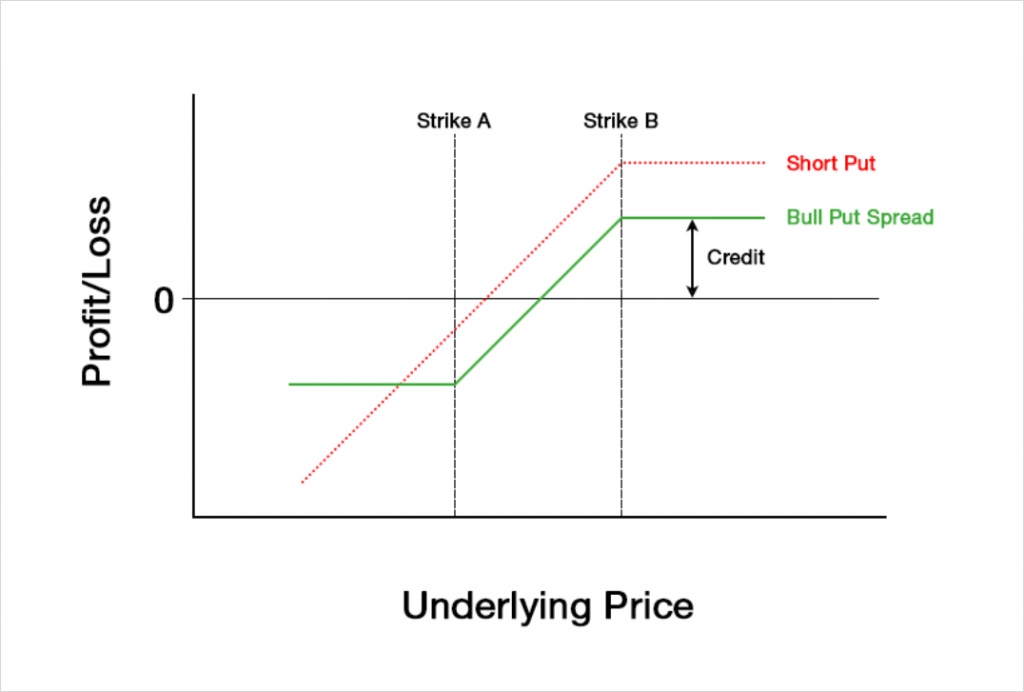
Just like when only selling a put option, the profit is capped. The maximum profit is limited to the net credit received. This occurs at expiry when the underlying price is higher than strike B.
Unlike when purchasing a put option, the risk of a bull put spread is also capped. This can be seen on the left side of the chart, where the P&L line flattens off again. This occurs at expiry when the underlying price is lower than strike A. It’s important to remember at this point that we are talking specifically about the dollar value of the payoff. This fixed risk property does not hold when we look at the payoff for the inverse contracts unless we make an adjustment, which we will come to later.
Selling a put option gives a trader a fixed reward, and a risk that is only capped by the underlying price reaching zero. By adding in the long leg at strike A, the bull put spread has capped the risk, meaning it’s now a fixed risk, fixed reward strategy. Obviously this change by itself is more desirable for the trader, so what is the catch? Because the put at strike A is purchased, the trader pays a debit for this leg, and although this debit will be smaller than the credit collected for the put at strike B, the total credit collected has been reduced. This reduction in credit moves the breakeven price higher, meaning that the underlying price has less room to fall before the trader starts to make a loss.
Compared to only selling a put, a bull put spread gives the trader a smaller potential profit, but it also caps their risk. They collect a smaller net credit, but once the price moves below strike A, the trader is no longer hurt by any further increases (at expiry at least).
The Greeks
We can add our Greek values for the put at strike A to the values for the put at strike B, and this will give us the total Greek values for the bull put spread.
To analyse how the Greeks behave we will need to assign some figures to each of the Black Scholes parameters. For today’s example of a bull put spread we will assume the following parameters:
Underlying price: $100
Time to expiry: 50 days
Interest rate: 0
Implied volatility: 60%
Strike A: $90
Strike B: $85
Profit and loss
With these parameters the $85/$90 bull put spread will initially give us a credit of about $1.56. The payoff chart looks like this.
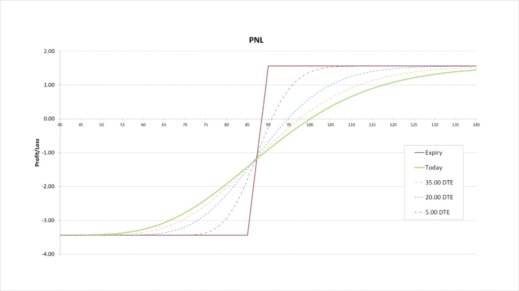
The maximum profit is capped at the net premium collected, which is $1.56. This maximum profit occurs when the underlying price is at or above the short strike of $90 at expiry.
The maximum loss is capped at the difference between the two strikes minus the net credit received. The difference between the long strike and the short strike is $5, and the net credit is $1.56, so the maximum loss for this trade is:
$5 – $1.56 = $3.44
The maximum loss occurs when the underlying price is at or below the long strike of $85 at expiry. It is this long strike at $85 that is capping our maximum loss compared to just being short the $90 put. We are effectively long the underlying between $90 and $85, but once $85 is breached to the downside, we are effectively flat again.
The breakeven can be calculated by subtracting the net credit collected from the strike price of the short put at $90. This gives us:
$90 – $1.56 = $88.44
This is exactly the same breakeven price as the bull call spread in the previous lecture.
Delta
As a bull put spread is a bullish trade that benefits from an increase in the underlying price, the total delta will be positive. We are short the $90 put, which gives us some positive delta. We are also long the $85 put which gives us some negative delta. Because the delta of the $90 put will always be of a larger magnitude than the delta of the lower strike $85 put, our total delta for a bull put spread will always be positive.
This chart shows the delta of the bull put spread, with the x axis being the underlying price. The extra lines also show how the delta will evolve as time passes.
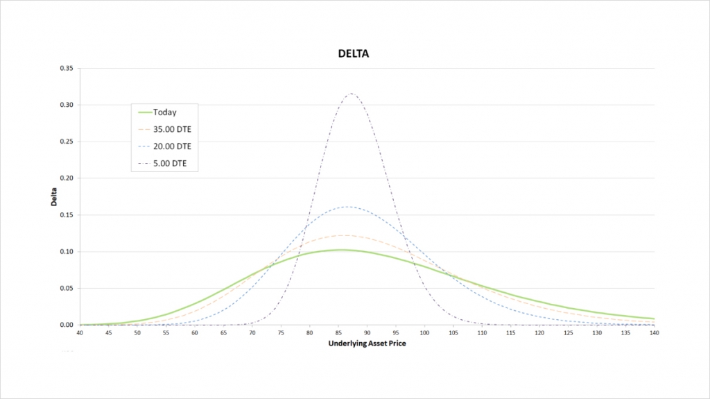
The delta of the bull put spread peaks around the long put strike of $85. Both put options will always have a delta of between 0 and -1, and the delta of the $90 strike will always be more negative than the delta of the $85 strike. As we are short the $90 strike, this means that the total delta for the bull put spread must be between 0 and 1. Due to the parameters chosen, they currently mostly cancel each other out though no matter where the underlying price moves, leading to a delta of considerably less than 1.
As time passes, the peak delta becomes more extreme, and the price range where there is any significant delta reduces significantly. As we come into expiry this effect accelerates. The peak delta can be seen when the short put at $90 is ITM, but the long put at $85 is still OTM. This is because as days to expiry (DTE) approaches 0, the delta of ITM puts approaches -1 and the delta of OTM puts approaches 0. Therefore, when the underlying price is between the two strikes as we are getting close to expiry, the delta our ITM short put is giving us is approaching 1, and the delta our OTM long put is giving us is approaching 0. This means our total delta is approaching 1.
The delta for the bull put spread then, is always positive, and peaks when the underlying price is between the two strikes. You may also notice that the shape of the delta chart for the bull put spread is almost identical to the delta chart for the bull call spread we looked at in lecture 12.2.
Gamma
As always, as we move from left to right on the delta chart, whenever the delta is increasing, this means the gamma is positive. Whenever the delta is decreasing, this means the gamma is negative. The steeper the line, the more extreme the gamma is.
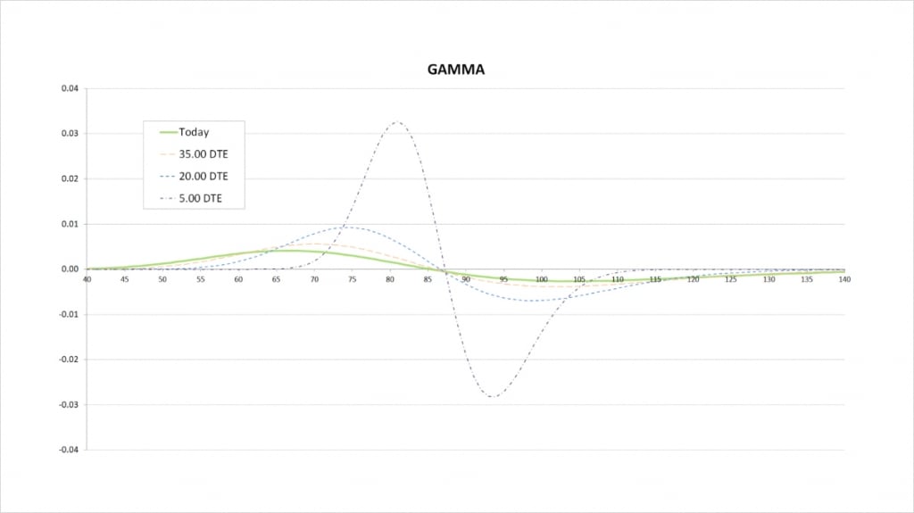
For the current values of delta with 50 days remaining until expiry, we see that delta increases slowly, peaks around the price of our long strike of $85, then increases slowly. On the gamma chart this is shown by gamma starting positive, then crossing the x axis at about the $85 strike, and then turning negative.
When we get much closer to expiry, the price range where there is any significant delta is much narrower, and delta changes much quicker. On the gamma chart this results in a narrower price range for significant gamma, and much more extreme values of gamma due to the more rapid changes in delta. The less time until the options expire, the closer the peaks in gamma will be to the strike prices of the options.
This gamma chart for the bull put spread is again very similar to that of the bull call spread.
Vega
We are long one put and short another put, so, as with the delta, we will always have one positive vega and one negative vega.
The magnitude of an option’s vega depends on where the underlying price currently is relative to the strike price of the option. Whether our bear put spread has negative or positive vega will therefore depend on where the underlying price is relative to the strikes.
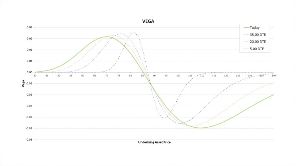
We are short the $90 put which gives us some negative vega, and we are long the $85 put which gives us some positive vega. To the left of the chart, we can see that because the $85 put is closer to the money, the positive vega we gain from this option outweighs the negative vega from the $90 put.
As we move to the point where both options are relatively close to the money, their vegas largely cancel each other out, giving the bull put spread a very small vega value.
Once we get to the right side of the chart, with the underlying price above both strikes, the $90 strike is closer to the money. This leads to the negative vega from being short the $90 strike outweighing the smaller positive vega we have from being long the $85 strike. The vega of the bull put spread is therefore negative here.
The less time is left until the options expire, the closer the underlying price has to be to our strike prices for the spread to have any significant vega. As we come into expiry, if both options are either far ITM or far OTM, then vega will be close to zero.
Theta
As with the gamma and vega, because we are long one put and short another put, we will always have one negative theta and one positive theta. Whether our bull put spread has negative or positive theta depends on where the underlying price is relative to the strikes.
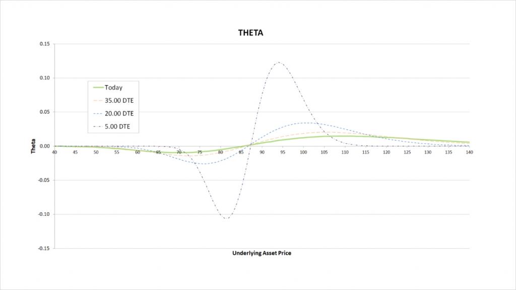
To the left of the theta chart, we can see that because the $85 put is closer to the money, the negative theta we have from this option outweighs the positive theta from being short the $90 put.
As we move to the point where both options are relatively close to the money, their thetas mostly cancel each other out, giving the bull put spread a very small theta value.
Once we get to the right side of the chart, with the underlying price above both strikes, the $90 strike is closer to the money. This leads to the positive theta from being short the $90 strike outweighing the smaller negative theta we have from being long the $85 strike. The theta of the bull put spread is therefore positive here.
The less time is left until the options expire, the closer the underlying price has to be to our strike prices for the spread to have any significant theta. As we come into expiry, if both options are either far ITM or far OTM, then theta will be close to zero.
Inverse option contracts
So far, everything we’ve looked at for the bull put spread, from the payoff in dollars to the shape of the Greek charts, has been extremely similar to what we saw in lecture 12.2 for the bull call spread.
When we look at how the payoff charts behave for inverse contracts, we see an important difference between how puts and calls behave.
This chart shows the bitcoin payoff at expiry of a bull put spread using the bitcoin options on Deribit. In this example we’ve sold one put option with a strike price of $44,000, and purchased one put option with a strike price of $40,000. We receive a credit of 0.06 BTC for the $44,000 put, and we pay a 0.04 BTC debit for the $40,000 put. This is the exact opposite of the bear put spread we discussed at the end of the previous lecture.
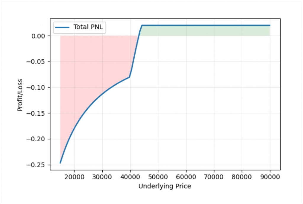
The most important thing to recognise, is that in bitcoin terms, the risk for this bull put spread is not fixed. We have added in a long put with a strike price of $40,000, which in dollar terms caps our risk, but in bitcoin terms it does not.
If the price expires below our long put strike of $40,000, we see that the loss in bitcoin continues to increase as the bitcoin price decreases. As the size of our long leg and short leg are the same here (both a size of 1), the dollar value of the maximum profit is still fixed, as it was in the dollar example earlier. The reason the maximum loss is not straight on the BTC payoff chart for the bull put spread though, is because as the underlying price of bitcoin decreases, the amount of bitcoin required to pay this fixed amount of dollars is increased.
For the bull put spread, when the underlying price expires below both strikes, this means that both puts are ITM. This means there is an intrinsic value that we need to pay out, and this value is first calculated in dollars, but then converted to and paid in bitcoin.
As an example, it takes twice as much bitcoin for us to pay the $4,000 value of the spread when the bitcoin price is at $20,000 (0.2 BTC), as it does when the bitcoin price is at $40,000 (0.1 BTC).
Defining fixed risk/reward with inverse contracts
Thankfully, it is still possible to fix both the risk and reward for the bull put spread in bitcoin terms. In this instance we need to pay out an increasing amount of bitcoin as the bitcoin price continues to decrease, so capping our risk in bitcoin terms instead would certainly be desirable.
The fact that our loss measured in bitcoin continues to increase as the price of bitcoin decreases, means we need to purchase more of the $40,000 strike puts. In doing so we will pay a larger debit for the long leg, but we will also limit our risk.
If we adjust our position sizing so that the ratio between the size of each of our two legs is the inverse of the ratio between the two strike prices, we achieve something that looks like this.
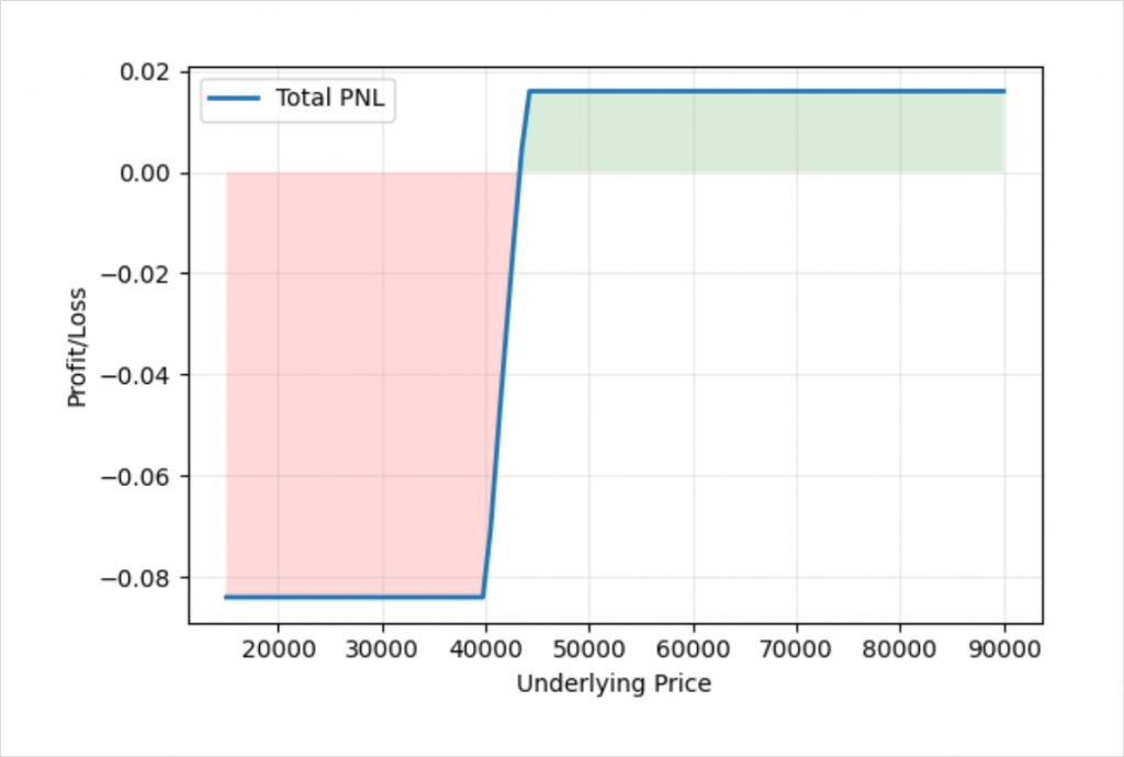
The ratio of the strike prices is:
40,000 : 44,000
Which is equal to:
1 : 1.1
If we invert this, we get a position sizing ratio that will set the risk to a fixed amount of bitcoin. This gives us a position sizing ratio of:
1.1 : 1
So if we buy the $40,000 put with a position size of 1.1, and sell the $44,000 put with a position size of 1, we get a position that is fixed risk and fixed reward in bitcoin terms, as desired.
Earlier we stated the prices of the $40,000 and $44,000 puts as 0.04 and 0.06 BTC respectively. When we execute the spread with a 1 : 1 ratio, this results in us receiving a net credit of 0.02 BTC. However when we execute the spread with a 1.1 : 1 ratio, we pay an extra debit of 0.004 BTC. This reduces our net credit for the spread to 0.016 BTC. So by adjusting the relative size of the two legs, we’ve reduced our maximum profit, but capped the maximum loss in BTC terms.
Vertical spreads
These first four lectures have looked at the four types of vertical spread. They’ve been a little repetitive because the strategies are so similar, so it may be useful to have a recap of the similarities and differences.
This table gives an overview of each of the strategies.
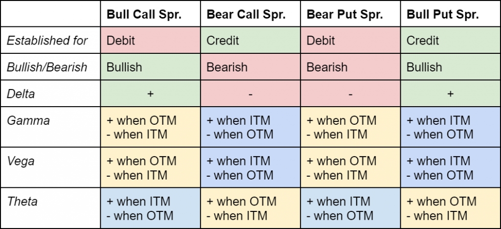
One thing to note is that if we choose strikes where both calls are OTM for example, the puts for those same strikes will by definition be ITM. Conversely if we choose strikes where both calls are ITM for example, then the puts for those same strikes will by definition be OTM. This means that we cannot simply flip our Greeks for a strategy on the same strikes by choosing puts over calls or vice versa.
A call spread and a put spread using the same strikes will theoretically have the same maximum profit/loss. If this were not the case, and there was a large enough difference, there would be an arbitrage opportunity. So whether to use puts or calls for a spread is normally going to be based on which has the best liquidity and tightest spreads. This will usually be with OTM options.
Vertical spreads offer traders the opportunity to cap their risk, and reduce the initial premium of a directional option trade. This does come at a cost though because the profit is also capped, so the trader will not gain anything extra from large moves in their favour. It is also important for traders of the inverse contracts on Deribit to be aware of how the profit/loss is calculated in the currency their account balance is in. This is particularly the case with a bull put spread, where the risk is capped in dollar terms but not in bitcoin terms (if trading the bitcoin inverse option contracts). It is however possible to adjust the vertical spreads to have fixed risk and reward in bitcoin terms by adjusting the sizing ratio between each leg.