


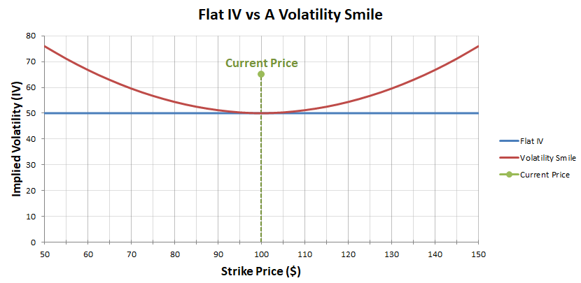
In the previous lecture we discovered that the IV levels are rarely the same for every strike price in a given expiration. When plotted on a chart, instead of a flat line, the volatilities create a curve, which is often in the shape of a smile.
We then saw a similar smile shape illustrated in a real world example when we looked at the IV of some options for SLV.
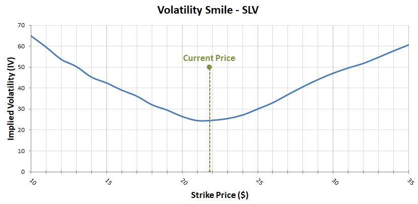
The lowest IV was with the ATM strikes around the current price. IV then increased in both directions in a relatively symmetrical fashion drawing a smile shape with the volatilities.
This isn’t the only shape the volatility curve can take though. This smile shape is often skewed to one side, and indeed the volatilities don’t always have to create a smile shape at all.
For example, the volatilities can create:
-A symmetrical smile, where OTM calls are priced roughly the same as OTM puts in volatility terms.
-Reverse skew, where lower priced options have higher IV, therefore OTM puts are priced higher than OTM calls. You may see this also referred to as a smirk (as opposed to a smile).
-Forward skew, where higher priced options have higher IV, therefore OTM calls are priced higher than OTM puts.
-Or even a frown, which would be the opposite of a smile, with the ATM options having the highest IV’s. In the real world you will almost never see a frown though.
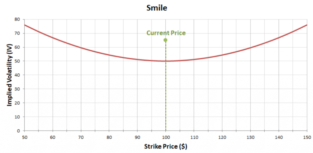
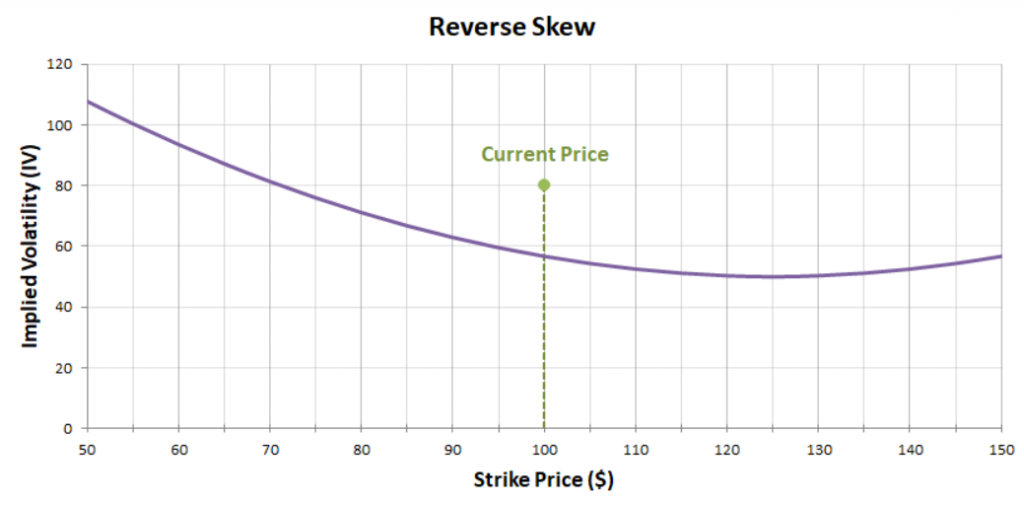
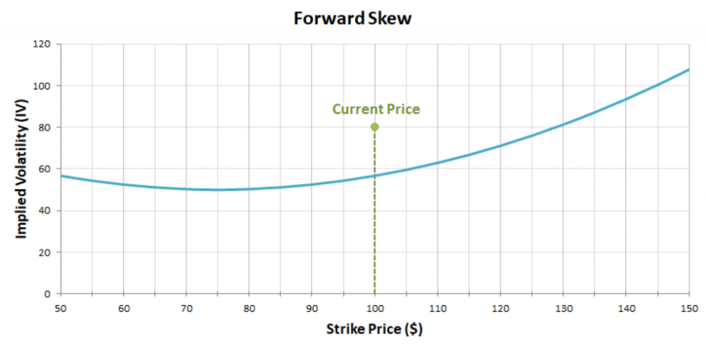
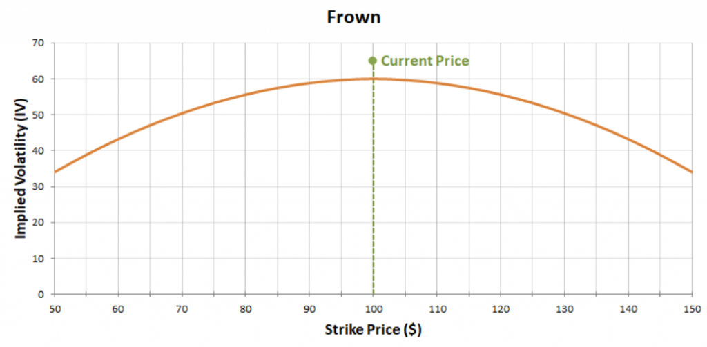
The actual percentages and prices used in these four charts are arbitrary examples, the shape of the curve is what we’re concerned with here.
Measuring skew
These different shapes are not fixed for any given asset, so it is useful to track the skew over time. A common way to measure skew is to subtract the IV of puts from the IV of calls. This results in a negative number when there is a reverse skew shape to the curve, and results in a positive number when there is a forward skew shape to the curve.
When making this comparison it is common to use the delta of the options, rather than the numerical distance from the strike price, to choose the specific options to compare. For example you may see a chart showing the 25 delta skew of an asset, which will be comparing the IV of a 25 delta call with the IV of a -25 delta put.
The deltas are actually 0.25 and -0.25 respectively, but there is a common convention to drop the decimal point when discussing deltas, and Quikstrike is doing this here. It’s also common to drop the sign when discussing the delta of a put option. So we might say a 25 delta put, when in reality the delta of the put is of course negative not positive.
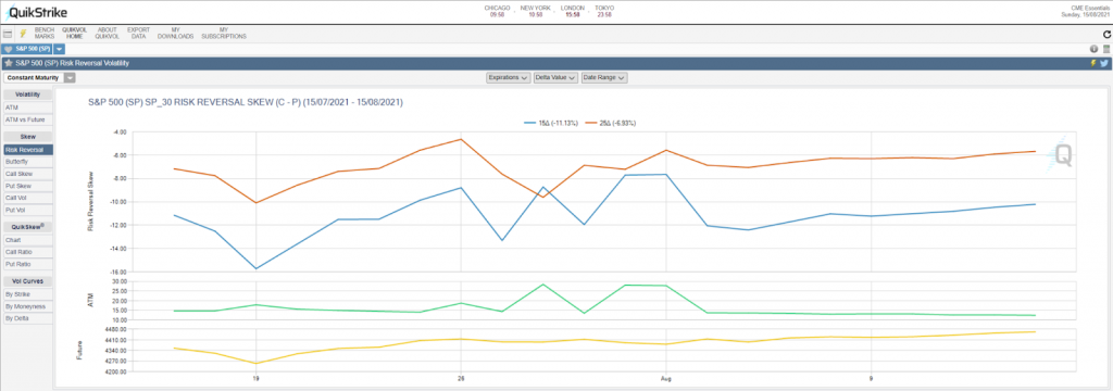
We can see an example of this by using an online tool called QuikStrike, which offers lots of useful option data and analysis tools. This is the free version that is available on the CME website. This chart is showing the 15 and 25 delta skews for the S&P 500. Rather than a specific expiration date, this is showing a constant maturity of 30 days, which is interpolated from the existing expiration dates.
In orange we can see the 25 delta skew, which is calculated as:
25 delta call IV – 25 delta put IV
Which in this case on the most up to date figure on the 13th of August, is currently equal to -5.68. This means that the IV of the 25 delta call is 5.68% lower than the IV of the 25 delta put, meaning the put is more expensive.
In blue we can see the 15 delta skew, which is calculated as:
15 delta call IV – 15 delta put IV
Which in this case, currently equals -10.22. This means that the IV of the 15 delta call is 10.22% lower than the IV of the 15 delta put, meaning the 15 delta put is even more expensive in volatility terms than the 15 delta call.
So S&P 500 option traders are valuing puts more than they are valuing calls. This is very common in this market, where underlying price decreases tend to be more volatile than price increases. It is also common for traders in this market to
-Purchase protection for their underlying long positions by purchasing puts as a type of insurance.
-Turn their underlying long position into a covered call by selling a call against it to earn a type of yield.
-Or, do both, by selling a call and buying a put, executing what’s known as a risk reversal or collar. We can see that this Quikstrike chart is actually labelled as Risk Reversal in the left menu, as it effectively shows how cheap or expensive a risk reversal that uses options with a particular delta is to execute.
While these won’t be the only strategies being executed of course, they are popular in this market, and each one has the effect of increasing put prices relative to calls.
Genesis Volatility Example
Similar skew charts are available for cryptocurrency options as well. Quickstrike does also have the same data available for bitcoin and ethereum, however at time of writing, they only use the CME options for the data, and so miss the larger volume and liquidity of Deribit.
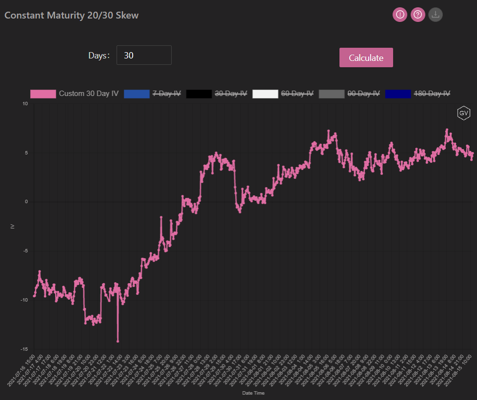
One site that focuses more on crypto options, is Genesis Volatility, which can be found at gvol.io. On this chart we are looking at the 30 day constant maturity skew. And for this chart on GVol, it uses all options with a delta between 0.2 and 0.3. So this will be similar, but not exactly the same as looking at the 25 delta skew like we saw on Quikstrike.
The skew is still calculated as:
Call IV – Put IV
But instead of using a specific option, an average implied volatility is calculated for all puts that have delta values between -.30 and -.20 and all calls with deltas between .20 and .30.
As we can see in this example, the skew in mid July was negative, meaning puts were more expensive than calls. During late June and early August though, this changed, and now in mid August, the skew is positive, meaning calls are more expensive than puts.
Summary
The volatilities will usually vary for each strike, even within the same expiration date. When plotted on a chart they will create a curve which is often skewed to one side.
It is possible to measure this skew by subtracting the IV of a put from the IV of a call. These options will usually have the same delta (except the put delta will be negative of course).
One very common measure of skew for example is to look at the 25 delta skew. This consists of a 25 delta call, and a 25 delta put (or deltas of 0.25 and -0.25 respectively if you prefer). This would be calculated as:
25 delta call IV – 25 delta put IV
When this is positive, calls can be said to be more expensive than puts. When this is negative, puts can be said to be more expensive than calls.